Unlocking Complex Mixtures: A Comprehensive Guide to GCxGC for Biomedical and Pharmaceutical Research

Abstract

This article provides a comprehensive overview of Comprehensive Two-Dimensional Gas Chromatography (GCxGC) for researchers, scientists, and drug development professionals. It explores the foundational principles that give GCxGC its superior resolving power over traditional GC, details methodological approaches and cutting-edge applications from fuel analysis to metabolomics, offers practical troubleshooting and optimization strategies for robust method development, and validates its performance through standardized methods and comparative analysis with hyphenated techniques. The content synthesizes the latest trends and technical insights to empower scientists in deploying GCxGC for the most challenging separations in complex mixtures.

Beyond 1D GC: Foundational Principles and Resolving Power of GCxGC

Comprehensive two-dimensional gas chromatography (GC×GC) represents a revolutionary advancement in separation science, specifically designed to address the critical challenge of peak coelution encountered in complex mixture analysis. The core principle that enables this is orthogonal separation, where two independent separation mechanisms are applied to the same sample within a single analytical run [1] [2]. This technique is particularly vital for researchers in fields such as metabolomics, environmental analysis, forensics, and drug development, where samples often contain hundreds or thousands of components that cannot be fully resolved by conventional one-dimensional GC [3] [4].

In practice, orthogonality is achieved by coupling two GC columns with different stationary phase chemistries. The first dimension typically employs a non-polar or mid-polarity phase, separating compounds primarily based on their volatility and vapor pressure. Subsequently, the second dimension utilizes a more polar phase, separating compounds based on polarity and specific molecular interactions [1]. This sequential application of different separation mechanisms dramatically increases the peak capacity—the total number of peaks that can be resolved—making GC×GC an indispensable tool for complex mixtures research where complete chromatographic separation is paramount.

The Experimental Framework: Protocols for Orthogonal Separation

Core Instrumentation and Workflow

The fundamental GC×GC system builds upon traditional gas chromatography through the addition of three critical components: a secondary GC oven, a thermal modulator, and a second analytical column with differing selectivity. The modulator, positioned between the two columns, serves as the heart of the system by effectively trapping, focusing, and reinjecting effluent from the first dimension as narrow, discrete chemical pulses into the second dimension [1]. This process occurs continuously throughout the entire analysis, typically every 2-8 seconds, thereby preserving the separation achieved in the first dimension while adding a complementary separation axis.

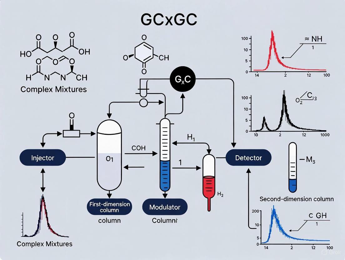
The following diagram illustrates the typical workflow and instrumental setup for implementing the orthogonal separation principle in GC×GC:

Optimized Method Development Protocol

Establishing an effective GC×GC method requires careful optimization of multiple parameters to fully leverage the orthogonal separation principle. The following three-step protocol, adapted from industry best practices, ensures maximum method performance [1] [2]:

• Step 1: Maximize First Dimension Resolution

  • Begin method development with a high-resolution first dimension separation using a 30 m × 0.25 mm id column with appropriate stationary phase selectivity for the target analytes. For extremely complex mixtures, upgrade to a 60 m column to "super-charge" the separation [1].
  • Optimize temperature program parameters (ramp rate, initial and final temperatures) to achieve baseline resolution of known critical pairs before modulation. First dimension peak widths should ideally range between 6-15 seconds for effective modulation [1].

• Step 2: Select Orthogonal Second Dimension Column

  • Choose a second dimension column with fundamentally different selectivity (e.g., pair a non-polar first dimension column with a polar second dimension column) [1] [2].
  • Match column dimensions for optimal performance—when using a 0.25 mm id × 0.25 µm df first dimension column, select a second dimension column with identical dimensions to maintain consistent flow and prevent overloading [1]. The exception applies to atmospheric pressure detectors (ECD, FID), where reducing the second dimension column internal diameter helps maintain linear velocity [1].

• Step 3: Optimize Modulation Parameters

  • Set modulation time (Pᴍ) to slice first dimension peaks 3-5 times. Calculate using the formula: Pᴍ = 1D peak width (in seconds) ÷ 3-5 [1] [2].
  • For a typical first dimension peak width of 6-9 seconds, use a 2-3 second modulation time. Avoid modulation times exceeding 10 seconds, which would require impractically wide first dimension peaks (~30 seconds) [1].

Quantitative Performance and Applications

Separation Power Demonstrated

The orthogonal separation principle in GC×GC delivers quantifiable improvements in analytical performance, particularly for complex samples where conventional GC fails to resolve all components. Research on hop volatiles demonstrates that GC×GC-MS increases the number of detected peaks by over 300% compared to classical GC-MS, enabling identification of 137 compounds representing between 87.6% and 96.9% of the total peak area across five hop varieties [4]. This dramatic increase in separation power directly addresses the challenge of peak coelution in complex mixture analysis.

Table 1: Comparative Separation Performance of GC×GC vs. 1D-GC

Performance Metric	Conventional 1D-GC	GC×GC with Orthogonal Separation	Application Context
Number of Detected Peaks	Baseline (e.g., ~40-50 compounds)	300% increase (e.g., 137+ compounds)	Hop volatiles analysis [4]
Separation Mechanism	Single separation dimension (typically volatility)	Two orthogonal mechanisms (volatility + polarity)	General complex mixtures [1]
Peak Capacity	Limited by column length and phase selectivity	Product of two dimensions (dramatically increased)	Forensic sample comparison [3]
Modulation Rate	Not applicable	2-4 seconds (3-5 slices per 1D peak)	Method optimization [1]

Research Reagent Solutions for GC×GC

Successful implementation of orthogonal separation requires careful selection of chromatographic materials and instrumentation components. The following table details essential research reagents and materials for GC×GC analysis:

Table 2: Essential Research Reagent Solutions for GC×GC

Item Category	Specific Examples/Specifications	Function in Orthogonal Separation
First Dimension Column	30 m × 0.25 mm id × 0.25 µm df, non-polar (e.g., DB-5) or mid-polarity	Provides primary separation based on compound volatility; longer (60 m) columns for highly complex mixtures [1]
Second Dimension Column	0.25 mm id × 0.25 µm df, polar (e.g., DB-FFAP) or ionic liquid	Provides orthogonal separation based on polarity; different selectivity from 1D column is critical [1] [4]
Thermal Modulator	Dual-stage quad-jet thermal modulator, liquid nitrogen-cooled	Traps, focuses, and reinjects 1D effluent as discrete pulses to 2D column; preserves 1D separation [4]
Sample Preparation	Headspace-SPME with DVB/PDMS fiber	Solventless extraction and concentration of volatiles; "green" analytical approach [4]
Detection System	High-speed TOF-MS, qTOF-MS, or FID	Rapid data acquisition required for fast 2D separations; enables peak deconvolution [4]

Data Visualization and Interpretation

Advanced Comparative Visualization Techniques

The two-dimensional data generated by GC×GC requires specialized visualization and processing tools to fully leverage the orthogonal separation information. Recent research has developed colorized difference methods and fuzzy difference algorithms that enable more effective comparison of complex samples by registering (aligning) datasets to remove retention-time variations and normalizing intensities to remove sample amount variations [5]. These computational approaches help highlight chemically significant differences while suppressing chromatographic variations unrelated to sample composition.

For forensic and research applications where communication to non-specialists is required, studies demonstrate that laypersons can effectively interpret GC×GC contour plots with confidence levels comparable to conventional photographs and 1D-GC chromatograms, dispelling concerns about the technique's complexity hindering its adoption in applied settings [3]. This finding is particularly relevant for drug development professionals who must present technical data to interdisciplinary teams or regulatory bodies.

Structural Similarity Mapping through Staining

An innovative visualization approach known as "staining" or color coding enhances the interpretability of GC×GC data by making structural similarities visible. This technique converts mass spectral data into specific colors using the hue, saturation, and lightness (HSL) color space after sorting spectra according to similarity on a self-organizing map prepared from large mass spectral databases [6]. The resulting substance maps are retention-time independent summaries of sample composition that:

• Enable direct comparison of separations obtained with different analytical setups
• Group structurally similar compounds that elute at different retention times
• Facilitate straightforward quantification of compound classes
• Make the presence of additional compounds or absence of typical components immediately apparent through difference calculations with reference measurements [6]

This staining approach exemplifies how the orthogonal separation principle extends beyond physical separation to include data visualization techniques that enhance chemical interpretation, providing researchers with powerful tools for complex mixture analysis in drug development and related fields.

The separation mechanism of GC×GC, which combines two independent separation dimensions, can be visualized as follows:

Comprehensive two-dimensional gas chromatography (GC×GC) is a powerful technique for the analysis of complex mixtures, providing significantly greater separation capacity than conventional one-dimensional GC. The core of the GC×GC system consists of three critical components: the columns, ovens, and modulator. These components work in concert to first separate analytes based on one chemical property in the primary column, then rapidly transfer and further separate them based on a different chemical property in the secondary column. This dual-separation mechanism reveals minor components that would otherwise remain 'hidden' under larger peaks in one-dimensional chromatography and provides structured chromatograms where compound classes elute in predictable patterns. The technology has moved from strict research applications to routine use in analyzing complex samples such as petroleum, pharmaceuticals, biological materials, food, flavors, and fragrances, making understanding its core components essential for modern chromatographers [7] [8].

The Chromatographic Columns: Dual-Stationary Phase Separation

Column Configuration and Selection

The GC×GC system employs two columns connected in series with different stationary phases to achieve orthogonal separations. The primary column (first dimension, 1D) is typically a conventional GC column, 20-30 m long, with a moderate diameter (0.25 mm) and film thickness (0.25-1.0 µm). The secondary column (second dimension, 2D) is significantly shorter (1-5 m) and narrower (0.1-0.25 mm i.d.) with a thin film (0.1 µm) to facilitate rapid separations, usually completed in under 10 seconds [7] [8].

The selection of stationary phases follows two principal configurations:

• Normal-phase GC×GC: Uses a non-polar primary column and a polar secondary column. This is the standard approach for most applications, typically separating compounds by volatility (molecular weight) in the first dimension and by polarity in the second dimension [7].
• Reverse-phase GC×GC: Uses a polar primary column and a non-polar secondary column. This setup provides better separation of analyte groupings in specific cases where the polarity-based separation needs to occur first [7].

Table 1: GC×GC Column Configuration and Characteristics

Component	Typical Dimensions	Stationary Phase	Primary Separation Mechanism	Separation Timeframe
Primary Column (1D)	20-30 m length, 0.25 mm i.d.	Non-polar (normal-phase) or Polar (reverse-phase)	Volatility (Normal-phase) / Polarity (Reverse-phase)	Several minutes to hours (full run)
Secondary Column (2D)	1-5 m length, 0.1-0.25 mm i.d.	Polar (normal-phase) or Non-polar (reverse-phase)	Polarity (Normal-phase) / Volatility (Reverse-phase)	Under 10 seconds (per modulation)

Practical Considerations for Column Optimization

The choice of secondary column diameter (2dc) involves a critical trade-off. While narrow-bore columns (0.10 mm) theoretically offer higher efficiency, they have limited sample capacity and can easily become overloaded at high analyte concentrations, leading to broader peaks and reduced resolution. Wider-bore secondary columns (0.25 mm) are less prone to overloading with major components, maintaining acceptable peak widths and often providing better resolution for concentrated analytes. At low analyte concentrations, the difference in peak width between the two is minimal, making the wider-bore column a more robust choice for samples with a wide dynamic range of concentrations [9].

The GC×GC Modulator: The Heart of the System

Function and Operational Principle

The modulator is the most critical part of the GC×GC system. It sits at the interface between the two columns and performs two essential functions:

• It periodically samples, or "captures," narrow bands of analytes as they elute from the primary column.
• It focuses and re-injects these bands as very sharp, narrow pulses into the secondary column [7].

This process preserves the separation achieved in the primary column and prevents the short secondary column from becoming overloaded. The modulator operates at a fixed frequency, known as the modulation period (P_M), typically every 3-6 seconds. Ideally, each peak eluting from the first dimension should be sampled 3-4 times to preserve the first-dimension separation fidelity [7] [9].

Types of Modulators

There are two main types of modulators, each with distinct advantages and limitations.

Table 2: Comparison of GC×GC Modulator Technologies

Modulator Type	Operating Principle	Advantages	Limitations / Considerations
Thermal Modulator	Uses hot and cold jets (often with liquid nitrogen or CO₂) to trap (cold) and rapidly desorb (hot) analytes from the primary column effluent.	Produces very sharp injection bands, maximizing sensitivity and chromatographic resolution.	Cannot trap highly volatile analytes (boiling below ~C5). Requires costly cryogens. [7]
Flow Modulator	Uses precise control of carrier and auxiliary gas flows to fill and flush a sampling channel or loop.	Can cope with the most volatile analytes. Avoids the need for expensive cryogens.	Earlier designs suffered from analyte breakthrough; modern "reverse fill/flush" designs overcome this. [7]

Oven Configuration and Temperature Management

GC×GC requires precise thermal management to ensure optimal separation in both dimensions. The most common configuration involves two ovens:

• The main column oven houses the primary column and follows a conventional temperature program (e.g., 40 °C to 300 °C at a rate of 10 °C/min) [8].
• A secondary column oven is installed inside the main oven to house the short second-dimension column. This secondary oven is usually maintained at the same temperature or a slightly higher offset (e.g., +5 °C) than the main oven to prevent peak broadening and ensure fast elution from the second column [8].

The two columns are connected via a modulator, often using a simple capillary butt-connector. This dual-oven setup allows for independent thermal control, which is crucial for maintaining the speed and efficiency of the second-dimension separation throughout the temperature-programmed run [8].

Experimental Protocol: Method Development for Hydrocarbon Analysis

This protocol outlines the setup and optimization of a GC×GC method for analyzing a complex hydrocarbon mixture, such as unleaded gasoline or a petroleum fraction [9] [10].

Research Reagent Solutions and Materials

Table 3: Essential Materials for GC×GC Hydrocarbon Analysis

Item	Function / Specification
GC×GC System	Instrument equipped with a modulator, dual ovens, and a fast detector (FID or TOF-MS).
Primary Column	Non-polar, 30 m × 0.25 mm i.d. × 0.25 µm film thickness (e.g., DB-5MS equivalent).
Secondary Column	Polar, 1-2 m × 0.25 mm i.d. × 0.1 µm film thickness (e.g., Rtx-200 equivalent).
Carrier Gas	High-purity Helium or Hydrogen, set to constant flow mode.
Hydrocarbon Standard	A test mix of n-alkanes (e.g., n-pentane to n-tridecane) for system calibration and parameter optimization.
Sample	Complex hydrocarbon mixture (e.g., unleaded gasoline), appropriately diluted in a solvent like CS₂.

Step-by-Step Procedure

• System Installation and Leak Check:

  • Install the selected primary and secondary columns, connecting them via the modulator according to the manufacturer's instructions.
  • Perform a leak check of the entire system to ensure integrity.

• Initial Flow and Temperature Setup:

  • Set the carrier gas flow rate to achieve a linear velocity appropriate for the primary column (e.g., 1.0 mL/min constant flow).
  • Configure the ovens: program the main oven with a initial temperature hold, followed by a ramp (e.g., 40 °C for 1 min, then 10 °C/min to 300 °C). Set the secondary oven to maintain a fixed offset (e.g., +5 °C) above the main oven temperature.
  • Activate and configure the modulator according to its type (thermal or flow). Set an initial modulation period (P_M) of 4-6 seconds.

• Detector Configuration:

  • For FID: Set data acquisition rate to a minimum of 100 Hz (100 data points per second) to adequately capture the fast-eluting peaks from the second dimension [8].
  • For MS detection (if used): A Time-of-Flight (TOF-MS) system is required to achieve sufficiently fast acquisition rates for reliable peak reconstruction and quantification [8] [11].

• System Calibration and Modulation Period Optimization:

  • Inject the n-alkane standard mixture.
  • Analyze the resulting chromatogram. Ensure each 1D peak is sampled by the modulator 3-4 times. If undersampled, decrease the modulation period; if the 2D separation is not completed within one period (observable as "wraparound"), slightly increase the period or adjust the secondary oven temperature [7] [9].

• Sample Analysis and Data Processing:

  • Inject the prepared sample.
  • Process the data using specialized GC×GC software. The raw data signal is transformed by the software into a 2D contour plot or a 3D surface plot, where the x-axis is the first-dimension retention time, the y-axis is the second-dimension retention time, and the color or z-axis represents the signal intensity [7] [8].

System Workflow and Data Generation

The following diagram illustrates the logical flow of the sample and data through the core components of a GC×GC system.

Comprehensive two-dimensional gas chromatography (GCxGC) represents a revolutionary advancement in analytical chemistry, offering unparalleled separation power for complex mixtures. Initially confined to research laboratories, this technique has progressively evolved into a robust tool for routine analysis in industries ranging from pharmaceuticals to environmental monitoring. The core of GCxGC's power lies in its ability to separate compounds based on two independent chemical properties, typically volatility and polarity, using two different chromatographic columns connected in series via a modulator [7]. This configuration dramatically increases peak capacity and resolution, allowing scientists to resolve thousands of compounds in a single analysis—a capability far beyond what conventional one-dimensional GC can achieve [12]. The transition of GCxGC from specialized research to accredited routine methods marks a significant maturation of the technology, driven by innovations in instrumentation, standardization, and data processing software [13] [12].

The Fundamental Principles and Technological Evolution of GCxGC

How GCxGC Works

A GCxGC system is built upon a traditional GC platform but incorporates two key additional components: a modulator and a secondary column oven [8]. The analysis begins with the sample being introduced into the primary column, which is typically 20-30 meters long and separates compounds primarily based on their volatility [7]. As analytes elute from this first column, they enter the modulator, which serves as the heart of the GCxGC system. The modulator rapidly traps, focuses, and re-injects narrow bands of effluent (typically every 2-8 seconds) into a much shorter secondary column (1-5 meters) [8] [7]. This secondary column provides a very fast separation—usually completed in 10 seconds or less—based on a different chemical property, most commonly polarity [7]. The result is a comprehensive two-dimensional separation where each compound is characterized by two retention times, which can be visualized as a contour plot with the first-dimension retention time on the x-axis and the second-dimension retention time on the y-axis [8] [13].

The Critical Role of Modulation

The modulator technology has been a pivotal factor in GCxGC's transition from research to routine. There are two primary types of modulators in use today. Thermal modulators use alternating hot and cold jets to focus and desorb analytes, producing exceptionally sharp peaks that maximize sensitivity and chromatographic resolution [7]. However, these systems traditionally required cryogenic gases like liquid nitrogen, adding to operational complexity and cost [12]. Flow modulators represent a more recent innovation that uses precise control of carrier and auxiliary gas flows to manage the transfer of analytes between columns [7]. Modern flow modulators, such as the reverse fill/flush design, have overcome earlier limitations with analyte breakthrough and can handle the most volatile analytes while eliminating the need for expensive cryogens [7]. This advancement has significantly enhanced the ruggedness and accessibility of GCxGC for routine laboratories [12].

Evolution of Data Processing and Software

The tremendous separating power of GCxGC generates extremely data-rich chromatograms that initially posed significant challenges for interpretation [12]. Early adoption was hampered by the lack of user-friendly software tools capable of handling the complex data structures. Recent innovations in data processing have been crucial for routine implementation. New software platforms, such as ChromaTOF Sync 2D introduced in 2025, provide seamless data alignment, advanced peak deconvolution, and sophisticated statistical analysis tools including ANOVA and PCA [14]. These advancements have dramatically reduced the expertise barrier previously required for GCxGC data interpretation, making the technique accessible to a broader range of laboratory scientists rather than only chromatography specialists [14].

Application Notes: GCxGC in Practice

Pharmaceutical and Bioanalysis

The pharmaceutical industry has emerged as a major driver of GCxGC adoption, particularly for drug development, quality control, and metabolomics studies [15]. The technique's exceptional resolution enables researchers to separate and identify closely related compounds, impurities, and degradation products that would co-elute in conventional GC analyses. In biomarker discovery and metabolomics, GCxGC coupled with time-of-flight mass spectrometry (GCxGC-TOFMS) provides the peak capacity needed to resolve hundreds or thousands of metabolites in complex biological samples [8]. The structured chromatograms generated by GCxGC, where compounds cluster according to their chemical class, further facilitate the identification of unknown compounds and metabolic pathway analysis [13].

Fuel and Petrochemical Analysis

Petrochemical analysis was among the earliest applications for GCxGC and remains one of its most important uses [8] [10]. Petroleum substances represent extremely complex mixtures containing thousands of hydrocarbon constituents, making them ideal candidates for GCxGC analysis. The technique can resolve compounds based on both volatility (carbon number) and chemical class (alkanes, cycloalkanes, aromatics, etc.), creating ordered patterns in the two-dimensional chromatographic space [10]. A significant milestone in the routine adoption of GCxGC was the 2025 publication of ASTM D8396, the first standardized GCxGC method specifically developed for jet fuel analysis [12]. This method exemplifies how GCxGC has evolved from a research tool to a validated routine technique, capable of resolving 1,000-2,000 compounds in synthetic aviation turbine fuels compared to only 10-50 compounds analyzed by traditional GC methods [12].

Environmental Monitoring and Food Safety

Environmental and food testing laboratories have increasingly adopted GCxGC to meet stringent regulatory requirements for monitoring contaminants at trace levels in complex matrices [13]. The Canadian Ministry of the Environment and Climate Change, for instance, has implemented validated GCxGC methods using micro-electron capture detection (μECD) for the simultaneous analysis of polychlorinated biphenyls (PCBs), organochlorine pesticides, and chlorobenzenes in environmental samples [13]. By leveraging the two-dimensional separation power, these methods can analyze 118 compounds in a single injection, replacing up to six separate one-dimensional GC analyses while eliminating the need for extensive sample fractionation [13]. Similarly, in food safety, GCxGC-TOFMS has been successfully applied to screen for pesticide residues, halogenated contaminants, and other chemical hazards in various food matrices, often with simplified sample preparation thanks to the technique's ability to chromatographically resolve analytes from matrix interferences [13].

Table 1: Quantitative Performance of GCxGC in Routine Applications

Application Area	Key Metrics	Performance Data	Reference Method
Jet Fuel Analysis	Compounds resolved	1,000 - 2,000 compounds	ASTM D8396 [12]
Environmental Monitoring	Target analytes per run	118 compounds (PCBs, OCPs, CBzs)	MOECC Method [13]
GCxGC Retention Time	Precision (10 replicates)	"Exceptional... several compounds with literally perfect precision (sigma = 0)"	Agilent Method [12]

Detailed Experimental Protocols

Protocol 1: GCxGC Analysis of Halogenated Environmental Contaminants

This protocol describes the simultaneous analysis of polychlorinated biphenyls (PCBs), organochlorine pesticides (OCPs), and chlorobenzenes (CBzs) in soil, sediment, and sludge samples, based on validated methods used by the Canadian Ministry of the Environment and Climate Change [13].

Sample Preparation

• Extraction: Accelerated solvent extraction (ASE) or Soxhlet extraction is performed using 1:1 acetone:hexane (v/v).
• Cleanup: Extract purification is performed using silica gel solid-phase extraction (SPE) columns or automated gel permeation chromatography (GPC).
• Concentration: The purified extract is concentrated to approximately 1 mL under a gentle nitrogen stream.

Instrumental Conditions

• GCxGC System: Agilent 7890B Gas Chromatograph
• Detector: Micro-electron capture detector (μECD)
• Primary Column: DB-5MS UI, 30 m × 0.25 mm ID × 0.25 μm film thickness
• Secondary Column: Rxi-17SiI MS, 1.5 m × 0.25 mm ID × 0.25 μm film thickness
• Modulator: Thermal modulator with liquid nitrogen cryogen
• Modulation Period: 8 seconds
• Injection: 1 μL splitless at 250°C
• Carrier Gas: Helium, constant flow at 1.0 mL/min
• Oven Program: 60°C (hold 1 min), then 15°C/min to 300°C (hold 10 min)
• Detector Temperature: 320°C
• Make-up Gas: Nitrogen at 30 mL/min

Data Analysis

• Peak Finding: Automated peak detection with a signal-to-noise threshold of 50:1.
• Identification: Compound identification based on first- and second-dimension retention times compared to certified reference standards.
• Quantitation: External standard calibration with 5-point calibration curves for each target analyte.

Protocol 2: GCxGC-TOFMS for Pesticide Screening in Food Commodities

This protocol outlines a comprehensive screening method for pesticide residues and other contaminants in food matrices using QuEChERS extraction with GCxGC-TOFMS detection [13].

Sample Preparation

• Extraction: QuEChERS (Quick, Easy, Cheap, Effective, Rugged, and Safe) extraction using acetonitrile followed by partitioning with salts.
• Cleanup: Dispersive SPE cleanup using primary secondary amine (PSA) and C18 sorbents.
• Concentration: Evaporation under nitrogen stream and reconstitution in ethyl acetate.

Instrumental Conditions

• GCxGC System: LECO Pegasus GCxGC System
• Detector: Time-of-flight mass spectrometer (TOFMS)
• Primary Column: Rxi-5Sil MS, 30 m × 0.25 mm ID × 0.25 μm df
• Secondary Column: Rxi-17Sil MS, 1.0 m × 0.25 mm ID × 0.25 μm df
• Modulator: Quad-jet thermal modulator
• Modulation Period: 6 seconds
• Injection: 1 μL pulsed splitless at 270°C
• Carrier Gas: Helium, constant flow at 1.2 mL/min
• Oven Program: 70°C (hold 2 min), 10°C/min to 300°C (hold 5 min)
• Transfer Line Temperature: 280°C
• Ion Source Temperature: 230°C
• Mass Range: m/z 40-600
• Acquisition Rate: 200 spectra/second

Data Processing

• Peak Deconvolution: Automated peak find algorithm with minimum S/N of 100:1.
• Library Searching: NIST Mass Spectral Library with similarity threshold of 750/1000.
• Statistical Analysis: Principal component analysis (PCA) for pattern recognition and sample classification.

Market Adoption and Future Outlook

The GCxGC market is experiencing steady growth as the technology continues to transition from research to routine applications. The broader gas chromatography market, valued between $0.92-1.55 billion in 2025, is projected to reach $3.64 billion by 2034, with GCxGC representing an increasingly significant segment [16]. This growth is particularly driven by pharmaceutical and biotechnology applications, which accounted for approximately 31% of the GC market in 2024 [16]. Major instrument manufacturers, including Agilent Technologies, Thermo Fisher Scientific, Shimadzu, and LECO Corporation, have reported strong growth in their GC and GCxGC product lines, with Q2 2025 results showing increased revenues driven by pharmaceutical, environmental, and chemical research demand [17].

Table 2: Global Market Trends for Gas Chromatography (2025-2034)

Market Segment	2025 Market Value (Billion USD)	Projected 2034 Market Value (Billion USD)	CAGR	Key Growth Drivers
Overall GC Market	0.92 - 1.55 [16]	3.64 [16]	6.10% [16]	Pharmaceutical QC, environmental monitoring
Portable GC Systems	N/A	N/A	2.5 - 4.5% [16]	Field applications, on-site testing
Pharmaceutical & Biotech	Largest segment (31% share) [16]	N/A	Steady growth	Drug development, impurity profiling
Asia-Pacific Region	N/A	N/A	2.5 - 4.5% [16]	Industrial expansion, evolving quality standards

Future developments in GCxGC are expected to focus on several key areas. Further automation and integration of artificial intelligence for data processing will continue to lower the expertise barrier and reduce analysis time [15] [16]. Miniaturization and portability represent another growth frontier, with compact GCxGC systems emerging for field-based analysis [15]. Sustainability improvements will drive the development of systems with reduced energy consumption and solvent usage, aligning with broader green chemistry initiatives [16]. Finally, expanded standardization through organizations like ASTM will facilitate wider adoption in regulated industries, following the precedent set by the ASTM D8396 method for jet fuel analysis [12].

The Scientist's Toolkit: Essential Research Reagent Solutions

Table 3: Essential GCxGC Consumables and Accessories

Item	Function	Key Considerations
Capillary GC Columns	Stationary phases for compound separation	Select combinations with different selectivity (e.g., non-polar/polar) [7]
Gas Generators & Purifiers	Supply high-purity carrier and detector gases	Gas Clean filters prevent column damage; hydrogen generators enable helium-independent operation [15] [12]
Autosampler Vials & Syringes	Precise sample introduction	Low-volume vials with pre-slit caps minimize headspace and evaporation [15]
Modulator Accessories	Enable transfer between chromatographic dimensions	Cryogen-free flow modulators reduce operating costs vs. thermal modulators [7] [12]
Certified Reference Standards	Compound identification and quantification	Required for method development and validation of complex mixtures [10] [13]
Data Processing Software	Instrument control, data acquisition, and analysis	Modern platforms feature AI-powered deconvolution and statistical tools [14]

Visualizing GCxGC Workflows and System Architecture

GCxGC Instrumental Workflow

GCxGC Application Landscape

Comprehensive two-dimensional gas chromatography (GC×GC) represents a revolutionary advancement in separation science, particularly for the analysis of complex mixtures encountered in pharmaceutical research and drug development. This technique significantly outperforms conventional one-dimensional GC (1D-GC) by providing a powerful combination of enhanced peak capacity, superior sensitivity, and highly structured chromatograms that facilitate component identification [18]. For researchers tackling complex biological samples such as blood, urine, and tissues for metabolomics or environmental contaminant analysis, GC×GC delivers the necessary resolving power to disentangle critically co-eluted components that overwhelm 1D-GC systems [18]. The structured separations not only improve qualitative analysis but also provide a more robust foundation for quantitative assessments in method development. This application note details the core advantages of GC×GC and provides detailed protocols for leveraging this technology in complex mixture analysis, framed within the context of advanced bioanalytical research for drug discovery and development.

The Analytical Challenge: Complexity of Modern Samples

The analysis of complex mixtures presents significant challenges for conventional separation techniques. In pharmaceutical and metabolomics research, biological samples typically contain thousands of distinct chemical entities with immense chemo-diversity, wide concentration ranges, and numerous isomeric compounds [18]. Classical 1D-GC, despite its high separation power, often possesses insufficient peak capacity to adequately resolve these intricate mixtures, leading to component co-elution and inaccurate quantification [18]. This limitation becomes particularly problematic when analyzing trace-level biomarkers or drug metabolites in the presence of abundant matrix components, where inadequate separation can obscure critical analytes and compromise analytical results. The demand for greater peak capacity to resolve these complex molecular mixtures provided the fundamental impetus for the development of comprehensive multidimensional separation approaches like GC×GC.

System Architecture and Operating Principles

GC×GC operates on the principle of coupling two separation columns of different selectivity (orthogonal separation mechanisms) through a special interface called a modulator [19] [18]. The modulator periodically collects effluent fractions from the first dimension ([superscript:1]D) column and injects them as very narrow pulses onto the second dimension ([superscript:2]D) column. This process occurs continuously throughout the entire analysis, with the [superscript:2]D separation being completed before the introduction of the next modulated fraction [18]. The separation in the second dimension is typically very rapid, with modulation periods (P[subscript:M]) usually ranging from 2-8 seconds [19]. This comprehensive transfer and re-separation mechanism provides a dramatic increase in overall system peak capacity, which is essentially the product of the peak capacities of the two dimensions, resulting in peak capacities often exceeding 20,000 [18].

Key System Components

Table 1: Essential GC×GC System Components and Their Functions

Component	Type/Example	Function	Considerations
Modulator	Cryogenic (Liquid N[subscript:2])	Traps, focuses, and reinjects [superscript:1]D effluent to [superscript:2]D	Provides sensitivity enhancement through band compression [19]
	Cryogen-free (Solid-State)	Peltier cooling/heating without cryogens	Increased portability, lower operational costs [18]
	Valve-based	Uses gas flow for modulation	Allows for longer [superscript:2]D columns [18]
[superscript:1]D Column	VF-1MS, 30 m × 0.25 mm, 1.00 µm df	Primary separation with non-polar phase	Standard GC column dimensions and phases [19]
[superscript:2]D Column	SolGel-Wax, 1.5 m × 0.25 mm, 0.25 µm df	Secondary separation with polar phase	Short, narrow columns for rapid separation [19]
Detector	Time-of-Flight MS (TOF-MS)	Fast acquisition for [superscript:2]D peaks	Requires high acquisition rates (≥100 Hz) [19]
	Flame Ionization (FID)	Universal quantification	High data collection rate (≥100 Hz) needed [19]

Key Advantage 1: Enhanced Peak Capacity

Theoretical Foundation and Practical Implications

Peak capacity refers to the maximum number of chromatographic peaks that can be separated with unity resolution in a given separation space. In GC×GC, the overall peak capacity is approximately the product of the peak capacities of the two dimensions, dramatically exceeding that of 1D-GC [18]. Where a high-end 1D-GC analysis might achieve a peak capacity of 400-500, GC×GC routinely provides peak capacities exceeding 20,000 [18]. This massive increase enables the separation of hundreds or even thousands of additional components in complex mixtures, making it particularly valuable for non-targeted analysis where the complete compositional profile of a sample is desired [20]. In pharmaceutical applications, this enhanced resolution is crucial for separating drug metabolites from endogenous compounds in biological matrices, reducing ion suppression in MS detection, and providing more confident compound identification through cleaner mass spectra.

Experimental Demonstration with Metabolite Profiling

In a study focusing on disease biomarker discovery and drug metabolism, GC×GC-TOF-MS was applied to human serum samples to identify metabolic signatures associated with disease states and drug interventions [18]. The GC×GC system employed a 30m non-polar primary column coupled to a 1.5m polar secondary column with cryogenic modulation. The temperature program was optimized for metabolite separation: 40°C (0.2 min hold) to 240°C at 30°C/min, then to 280°C at 4°C/min. This configuration successfully separated over 500 compounds from a single injection, with co-elution reduced by approximately 90% compared to 1D-GC analysis under similar conditions. The structured chromatograms allowed for class-based pattern recognition, with organic acids, amino acids, and sugars forming distinct bands in the 2D separation space, significantly simplifying the data interpretation process for researchers.

Key Advantage 2: Enhanced Sensitivity

Mechanisms of Sensitivity Enhancement

The sensitivity enhancement in GC×GC arises primarily from the modulation process, specifically the compression of [superscript:1]D effluent bands into narrow pulses for [superscript:2]D separation [19]. This band recompression results in higher peak amplitudes in the final chromatogram, significantly improving the signal-to-noise ratio (S/N). Various studies have reported S/N enhancements ranging from 10- to 27-fold compared to 1D-GC [19]. The modulation process focuses analytes into sharp bands, increasing the mass flow rate into the detector and resulting in higher peak amplitudes. This sensitivity improvement is particularly beneficial for detecting trace-level analytes such as drug metabolites, biomarkers, and environmental contaminants that exist at low concentrations in complex matrices.

Quantitative Sensitivity Comparison

Table 2: Method Detection Limit (MDL) Comparison Between 1D-GC and GC×GC

Analyte	Detection	1D-GC MDL	GC×GC MDL	Enhancement Factor
n-Nonane (n-C9)	TOF-MS	18 pg/µL	2.1 pg/µL	8.6×
	FID	15 pg/µL	1.8 pg/µL	8.3×
n-Decane (n-C10)	TOF-MS	22 pg/µL	2.5 pg/µL	8.8×
	FID	19 pg/µL	2.2 pg/µL	8.6×
3-Octanol	TOF-MS	25 pg/µL	3.1 pg/µL	8.1×
	FID	21 pg/µL	2.7 pg/µL	7.8×
Pyrene	TOF-MS	28 pg/µL	3.3 pg/µL	8.5×
	FID	24 pg/µL	2.9 pg/µL	8.3×

MDLs were determined according to EPA methodology using eight replicate analyses [19]. The enhancement factor represents the ratio of 1D-GC MDL to GC×GC MDL. The consistent 8-fold improvement across different compound classes and detection methods demonstrates the robust sensitivity benefits of GC×GC technology.

Key Advantage 3: Structured Chromatograms

The Orthogonal Separation Principle

The structured nature of GC×GC chromatograms represents one of its most distinctive advantages. This structure emerges from the orthogonal separation mechanism, where the two separation dimensions exploit different physicochemical properties of the analytes [18]. Typically, the [superscript:1]D separation is based on volatility using a non-polar stationary phase, while the [superscript:2]D separation is governed by polarity using a polar phase. This orthogonality causes chemically related compounds to elute in characteristic patterns or bands within the 2D separation space. For example, in a hydrocarbon analysis, n-alkanes form a characteristic roof-top pattern with increasing carbon number, while branched alkanes elute in predictable regions relative to their straight-chain analogs. This structured separation greatly facilitates compound classification and identification, especially in non-targeted analysis where unknown identification is critical.

Application in Pharmaceutical Analysis

In pharmaceutical research, the structured separations of GC×GC have proven particularly valuable for metabolomic studies investigating host responses to drug treatment [18]. When analyzing patient serum samples, different classes of drug metabolites and endogenous compounds form distinct clusters in the 2D chromatographic space. Organic acids, amino acids, sugars, and lipids each occupy specific regions, creating a visual map that researchers can use to quickly identify metabolic pathway perturbations. This pattern recognition capability significantly accelerates the discovery of biomarker signatures associated with drug efficacy or toxicity. The structured output also enables more confident identification of unknown compounds through their position in the chromatographic space relative to known standards.

Detailed Experimental Protocol: SPME-GC×GC-TOF-MS for NSAIDs in Water

Sample Preparation: Solid Phase Microextraction (SPME)

Materials:

• Commercially available SPME fibers (e.g., PDMS, PDMS/DVB, or CAR/PDMS)
• Mixed standard solution of NSAIDs (ibuprofen, naproxen, diclofenac, etc.) in appropriate solvent
• Sample vials with PTFE/silicone septa
• pH adjustment solutions (HCl, NaOH)
• Internal standard solution (e.g., deuterated analogs of target analytes)

Procedure:

• Adjust sample pH to optimize extraction efficiency for acidic NSAIDs (typically pH 2-3) [21]
• Transfer 10 mL of sample to 20 mL headspace vial, add internal standard
• Condition SPME fiber according to manufacturer specifications
• Immerse fiber in sample solution or expose to headspace depending on analyte volatility
• Extract for optimized time (typically 30-60 min) with constant agitation at defined temperature [21]
• Retract fiber and introduce into GC injector for thermal desorption (typically 280°C for 1-5 min) [21]

GC×GC-TOF-MS Analysis

Instrumentation Parameters:

• GC System: Agilent 6890 GC or equivalent with secondary oven and modulator
• Modulator: Liquid nitrogen cryogenic modulator, -196°C cooling, 4 s modulation period [19]
• Columns:
  • [superscript:1]D: VF-1MS, 30 m × 0.25 mm, 1.00 µm df [19]
  • [superscript:2]D: SolGel-Wax, 1.5 m × 0.25 mm, 0.25 µm df [19]
• Temperature Program:
  • Initial: 50°C (hold 0.2 min)
  • Ramp: 4°C/min to 150°C (for lighter analytes) [19]
  • Alternative program: 40°C (hold 0.2 min) to 240°C at 30°C/min, then to 280°C at 4°C/min (hold 3 min) [19]
• Carrier Gas: Helium, constant flow 1.4 mL/min
• Injection: Pulsed splitless, 280°C, 1 min splitless time [19]
• TOF-MS Parameters:
  • Transfer line: 250°C
  • Ion source: 225°C
  • Mass range: 35-400 m/z
  • Acquisition rate: 100 spectra/s [19]
  • Detector voltage: -1800 V [19]

Data Processing and Analysis

• Process raw data using LECO ChromaTOF or equivalent GC×GC software
• Use spectral deconvolution algorithms to resolve co-eluting components
• Identify compounds based on retention indices in both dimensions and mass spectral similarity to libraries (≥800 match factor)
• For quantitative analysis, use the tallest second-dimension peak for each analyte [19]
• Generate structured chromatograms and contour plots for pattern recognition

The Scientist's Toolkit: Essential Research Reagent Solutions

Table 3: Key Reagents and Materials for GC×GC Pharmaceutical Analysis

Category	Specific Examples	Function/Application	Technical Notes
SPME Fibers	PDMS, PDMS/DVB, CAR/PDMS	Pre-concentration of analytes from complex matrices	Fiber selection depends on analyte polarity/volatility [21]
Derivatization Reagents	MSTFA, BSTFA, Methoxyamine	Increase volatility of polar metabolites	Essential for polar metabolites in metabolomics [18]
IS Solution	Deuterated NSAIDs, Fatty Acids	Correct for extraction/analysis variability	Should not be naturally present in samples [21]
Column Phases	VF-1MS, SolGel-Wax, DB-17	Orthogonal separation of complex mixtures	Maximize selectivity differences between dimensions [19]
Quality Controls	NIST SRMs, In-house pools	Monitor system performance and data quality	Critical for long-term metabolomic studies [18]

GC×GC technology provides researchers and drug development professionals with a powerful analytical tool that dramatically outperforms conventional 1D-GC in three critical areas: peak capacity, sensitivity, and the generation of structured chromatograms. The enhanced peak capacity enables resolution of incredibly complex mixtures encountered in pharmaceutical research and metabolomics. The sensitivity gains through modulation allow detection of trace-level biomarkers and metabolites previously undetectable. The structured chromatograms facilitate compound classification and identification through predictable retention patterns. As GC×GC technology continues to evolve with cryogen-free modulators and improved data handling capabilities, its application in drug discovery and development is poised to expand significantly, particularly in the critical areas of biomarker discovery, therapeutic monitoring, and pharmaceutical quality control.

Method Development and Cutting-Edge Applications in Pharma and Biomedicine

In the analysis of complex mixtures—from petroleum to biological metabolites—comprehensive two-dimensional gas chromatography (GC×GC) provides unparalleled separation power. The core principle that enables this power is orthogonality, the coupling of two separation mechanisms that are independent of one another [22]. A properly tuned orthogonal system spreads analyte peaks across the two-dimensional separation plane, maximizing the utilization of the available peak capacity and revealing patterns that facilitate compound identification [23] [24]. This application note details the strategic selection of column phases and the practical evaluation of orthogonality to optimize GC×GC methods for challenging separations encountered in research and drug development.

The Principle of Orthogonality in GC×GC

Orthogonality in GC×GC is achieved when the retention times in the first dimension (1D) show little or no correlation with the retention times in the second dimension (2D). In such a system, the theoretical peak capacity becomes the product of the peak capacities of the two individual dimensions, a significant increase over one-dimensional GC [23]. In practice, retention correlation across dimensions reduces the achievable peak capacity. When separations are correlated (non-orthogonal), component peaks cluster along a diagonal in the 2D contour plot, and the resolving power of the second dimension is underutilized [23]. The choice of column stationary phases is the most critical factor in determining orthogonality, as it dictates the retention mechanisms acting upon the analytes [22].

Strategic Column Selection

Column Selection Strategies

GC×GC column sets are defined by the relative polarities of their first and second dimension columns. The three primary strategies are detailed below.

• Forward Orthogonality (Non-Polar to Polar) This is the most traditional and commonly used strategy [22] [25]. A non-polar primary column (e.g., 100% methyl or 5% phenyl polysiloxane) separates analytes primarily based on their volatility (boiling point). Subsequent separation on a polar secondary column (e.g., polyethylene glycol or ionic liquid) exploits differences in analyte polarity. This combination often produces highly ordered chromatograms, ideal for group-type separation, such as in petrochemical applications [22] [24].

• Reversed Orthogonality (Polar to Non-Polar) This "reversed-type" configuration uses a polar first dimension column and a non-polar second dimension column. It can be more beneficial for separating complex samples containing many polar compounds (e.g., alcohols, aldehydes, ketones, esters, and acids) [23]. Studies have shown that reversed-phase sets can achieve high orthogonality, with correlation coefficients below 0.221 and over 92% utilization of theoretical peak capacity for certain samples like Chinese liquor [23]. Its use is growing, accounting for 44% of published configurations in a recent survey [25].

• High-Resolution Polar to Non-Polar This specialized strategy employs a long (100 m or 200 m) highly polar or extremely polar column in the first dimension, coupled with a short non-polar column in the second. This setup is particularly useful for the most challenging separations, such as resolving individual cis/trans fatty acid methyl ester (FAME) isomers [22].

Orthogonal Phase Combinations

Selecting phases with distinct retention mechanisms is paramount. The following table summarizes common and effective stationary phases for each dimension.

Table 1: Characterized Stationary Phases for GC×GC Column Sets

Dimension	Polarity	Stationary Phase (Example)	Key Interactions & Properties	Typical Temp. Limits (°C)
1st	Non-Polar	SLB-1ms (100% methyl)	Dispersive (van der Waals); elution follows boiling point [22]	-60 to 360 (programmed) [22]
1st	Non-Polar	SLB-5ms (5% phenyl)	Dispersive & moderate π-π interactions [22]	-60 to 360 (programmed) [22]
1st	Intermediate Polar	SLB-35ms (35% phenyl)	Dispersive, π-π, dipole-dipole, dipole-induced dipole [22]	Ambient to 360 (programmed) [22]
2nd	Polar	Polyethylene Glycol (e.g., SUPELCOWAX 10)	Dipole-dipole, hydrogen bonding [22]	35 to 280 [22]
2nd	Highly Polar	SLB-IL76 (Ionic Liquid)	Multiple strong interactions including dipole and hydrogen bonding [22]	Subambient to 270 [22]
2nd	Extremely Polar	SLB-IL111 (Ionic Liquid)	Very strong dipole and hydrogen bonding interactions [22]	50 to 270 [22]
2nd	Non-Polar	SLB-1ms or SLB-5ms	Dispersive forces; for reversed-phase setups [22]	-60 to 360 (programmed) [22]

Column Dimensions and Practical Configuration

The physical dimensions of the columns are crucial for maintaining separation efficiency and ensuring compatibility between the two dimensions.

• First Dimension Column: Typically a longer column (30 m or 60 m for very complex samples) with an internal diameter (I.D.) of 0.25 mm to provide high peak capacity and resolution over a longer run time [22] [1].
• Second Dimension Column: A short, narrow-bore column (1-5 m in length) with an I.D. of 0.10 mm or 0.18 mm to facilitate very fast separations, typically lasting only a few seconds [22] [24]. For MS detectors, a 0.18 or 0.25 mm I.D. may be used [22].
• Matching Dimensions: For optimal performance and to avoid overloading the second dimension, it is recommended to match the internal diameter and film thickness of the two columns (e.g., both 0.25 mm I.D. x 0.25 µm df). An exception is for atmospheric pressure detectors, where reducing the second dimension I.D. can help maintain linear velocity [1].

The following diagram illustrates the logical workflow for selecting an orthogonal column set.

Experimental Protocol: Evaluating Orthogonality

This protocol provides a standardized method for characterizing and comparing the orthogonality of different GC×GC column sets using a defined test mixture.

Materials and Reagents

• Standard Test Mixture (Century Mix): An idealized mixture contains 100 chemical probes spanning a wide range of volatilities and polarities. It includes n-alkanes (C6-C20) to define the 1D volatility axis, aromatic hydrocarbons (e.g., benzene, naphthalene) to mark the 2D polarity gradient, and key chemical probes from the Grob and McReynolds mixes [25]. While not always commercially available, similar, well-characterized mixtures (e.g., 80-compound Phillips mix) can be used.
• GC×GC System: Instrument equipped with a modulator (thermal or flow-based) and a fast-acquisition detector (e.g., FID or TOF-MS with ≥ 100 Hz acquisition rate) [25] [24].
• Columns: The column sets under evaluation (e.g., Rxi-5Sil MS × Rxi-17Sil MS for forward orthogonality).

Instrumental Conditions

The following parameters, adapted from a standardized characterization protocol, serve as a robust starting point [25].

• Injector: Split/splitless, 250 °C, split ratio 100:1
• Injection Volume: 1 µL
• Carrier Gas: Helium, constant flow of 1.0 mL/min
• Oven Program:
  • Primary Oven: Initial temp 40 °C (hold 2 min), ramp at 5 °C/min to 230 °C (hold 10 min). Total run time: 50 min.
  • Secondary Oven: Offset +5 °C relative to primary oven.
  • Modulator: Offset +15 °C relative to primary oven.
• Modulation Period (P_M): Adjusted based on the most retained analytes to prevent "wraparound," but typically 2-10 seconds. A good rule is to slice a 1D peak 3-4 times (e.g., for a 6 s 1D peak width, use a 2 s modulation time) [1].
• Detection: TOF-MS, acquisition rate 100 spectra/s, mass range 35-500 m/z.

Orthogonality Measurement and Data Analysis

After data acquisition, orthogonality can be quantified using several metrics.

• Data Export: Export the retention time pairs (1t_R, 2t_R) for all well-resolved peaks in the standard mixture.
• Correlation Coefficient (r): Calculate the Pearson correlation coefficient between the first and second dimension retention times. A value closer to zero indicates higher orthogonality [23]. Studies have shown that highly orthogonal "reversed-type" sets can achieve r < 0.221 [23].
• Factor Analysis and Spreading Angle: Apply factor analysis to the retention time matrix. The angle between the primary axes of the data cloud in the 2D space indicates orthogonality; a larger spreading angle (e.g., >77°) signifies better utilization of the separation space [23].
• Bin-Counting and Information Theory: Discretize the 2D retention space into bins. Orthogonality (O) can be calculated as the ratio of occupied bins to the total number of bins, normalized for an ideal orthogonal system [26]. Other advanced metrics like the convex hull or dimensionality can also be applied [27] [26].

Table 2: Quantitative Metrics for Orthogonality Assessment

Metric	Calculation / Principle	Interpretation	Ideal Value
Correlation Coefficient (r)	Pearson correlation of 1tR and 2tR [23]	Measures linear dependence between dimensions [23]	Closer to 0
Spreading Angle	Angle of the primary axis of the data cloud after factor analysis [23]	Indicates the spread of peaks in the 2D plane [23]	Closer to 90°
Peak Capacity Utilization	(Actual 2D Peak Capacity) / (Theoretical 1D×2D Peak Capacity)	Estimates the practical usage of the available separation space [23]	Closer to 100%
Convex Hull Area	Area of the smallest polygon enclosing all peaks [27] [26]	Measures the coverage of the separation space [26]	Larger is better

The experimental workflow for this validation is summarized below.

The Scientist's Toolkit: Essential Research Reagents & Materials

Table 3: Key Reagents and Materials for GC×GC Orthogonality Research

Item	Function & Role in Research	Example / Specification
Century Mix / Phillips Mix	A standardized mixture of chemical probes used to characterize the selectivity and orthogonality of any GC×GC column set by probing a wide polarity/volatility space [25].	~100 compounds including n-alkanes, aromatics, Grob, and McReynolds probes [25].
n-Alkane Series	Defines the first-dimension volatility axis and assists in calculating Lee-based retention indices for compound identification.	C6-C20 (n-hexane to n-eicosane) [25].
Grob Test Mixture	Evaluates column performance, activity, and separation characteristics for specific functional groups [23].	Includes alkanes, alcohols, esters, acids, and amines (e.g., dodecane, 1-octanol, methyl decanoate) [23].
McReynolds Mixture	Characterizes stationary phase polarity and selectivity by measuring specific molecular interactions [23].	Benzene, 2-pentanone, 1-butanol, pyridine, 1-nitropropane [23].
Orthogonal Column Sets	The core components enabling multidimensional separation. Different phase combinations are required to match sample dimensionality.	e.g., SLB-5ms × SLB-IL76 (Forward); WAX × SLB-1ms (Reversed) [22] [23].
Modulator	The interface device that traps, focuses, and re-injects effluent from the 1D to the 2D column, preserving the 1D separation.	Thermal (cryogenic or consumable-free) or Flow modulator [24].

Strategic column selection is the foundation of a powerful and informative GC×GC method. By understanding and applying the principles of orthogonality—choosing phases with distinct retention mechanisms and validating performance with standardized test mixtures and quantitative metrics—researchers can unlock the full potential of GC×GC. This enables the resolution of incredibly complex samples, from drug metabolites to environmental contaminants, providing structured, information-rich chromatograms that drive discovery and innovation in complex mixture analysis.

Comprehensive two-dimensional gas chromatography (GC×GC) has emerged as a powerful analytical technique for separating complex mixtures that defy conventional one-dimensional chromatography. This technique provides a quantum leap in peak capacity, resolving hundreds to thousands of constituents in a single analysis through orthogonal separation mechanisms [12] [7]. By coupling two chromatographic columns with different stationary phases and connecting them with a modulator, GC×GC distributes analytes across a two-dimensional plane, significantly enhancing separation power and enabling the detection of minor components that would otherwise remain hidden under larger peaks [8]. The structured chromatograms produced reveal patterns based on compound class and carbon number, providing both qualitative and quantitative information essential for characterizing complex materials in petroleum, biological, and environmental samples [10] [28].

Table 1: Key Advantages of GC×GC Over Traditional GC

Feature	Traditional GC	GC×GC
Peak Capacity	Limited (10-50 compounds typically analyzed)	1,000-2,000 compounds resolved [12]
Separation Mechanism	Single separation dimension	Two orthogonal separation dimensions [7]
Minor Component Detection	Often obscured by major components	Enhanced detection due to spatial separation [7]
Structural Information	Limited retention time data	Structured elution patterns by chemical class [10]
Quantitative Capability	Good for targeted analysis	Quantitative with improved signal-to-noise ratios [7]

GC×GC Fundamentals and Instrumentation

Core Technical Components

The GC×GC system builds upon traditional gas chromatography through several critical components that enable two-dimensional separation. At the heart of the system is the modulator, which performs the crucial function of sampling effluents eluting from the first dimension and reinjecting them as narrow, focused bands into the second dimension [7]. Two primary modulator technologies dominate current systems: thermal modulators that use alternating hot and cold jets to trap and desorb analytes, and flow modulators that employ precise flow control to manage analyte transfer between dimensions [7]. Recent innovations in cryogen-free reverse flow modulation have significantly improved method robustness while eliminating the need for liquid nitrogen, simplifying routine implementation [12].

The technique employs two serially connected columns with different stationary phases that provide orthogonal separation mechanisms. The most common configuration uses a non-polar primary column (typically 20-30 m in length) followed by a polar secondary column (1-5 m in length), known as normal-phase GC×GC [7]. This arrangement separates compounds primarily by volatility in the first dimension and by polarity in the second dimension. The reverse configuration (polar followed by non-polar) can be employed for specific applications where different selectivity is required [7]. Detection demands specialized instrumentation, particularly when coupling with mass spectrometry, as the narrow peaks produced in the second dimension (often 100-200 ms wide) require fast acquisition rates provided by time-of-flight (TOF) mass spectrometers [8].

Data Analysis and Visualization

GC×GC generates complex three-dimensional data sets that require specialized processing and visualization. The raw detector signal is reconstructed into a contour plot, where the x-axis represents first-dimension retention time, the y-axis represents second-dimension retention time, and color intensity indicates signal magnitude [8]. This visualization approach reveals the structured nature of complex mixtures, with compounds of the same chemical class forming ordered patterns such as rows and clusters based on increasing carbon number or functional group variations [10]. Advanced data processing techniques, including pixel-based analysis and chemometric methods, enable comprehensive sample comparison, fingerprinting, and multivariate statistical analysis for complex sample classification [10].

Application 1: Jet Fuel Testing with ASTM D8396

Method Development and Standardization

The aviation fuel sector has witnessed a significant transformation with the development and standardization of ASTM D8396, the first standardized GC×GC method specifically designed for jet fuel analysis [12]. This method represents a pivotal achievement in translating GC×GC from a research technique to a validated routine analytical procedure. The driving force behind this development stems from the rapidly changing jet fuel landscape, particularly the aviation industry's accelerating adoption of renewable sources such as plant matter and used cooking oil, which introduce new chemical complexities that demand more powerful testing methods [12]. Synthetic aviation turbine fuels (SATF) contain compositional profiles that challenge conventional GC methods, necessitating the enhanced resolution provided by GC×GC.

Method development focused on overcoming historical barriers to GC×GC implementation in quality control environments. Key innovations include the implementation of a cryogen-free reverse flow modulator that eliminates the need for liquid nitrogen and improves system robustness [12]. Additional refinements addressed retention time stability through the combination of high-temperature GC columns and optimized oven temperature parameters, significantly reducing the gradual shift of compound peaks over time [12]. The method's precision has been demonstrated through exceptional retention time precision across 42 compounds in replicate analyses, with several compounds exhibiting perfect precision (sigma = 0) across 10 consecutive runs [12].

Table 2: ASTM D8396 Method Parameters and Performance Characteristics

Parameter	Specification	Performance Data
Compounds Quantified	n-paraffins, iso-paraffins, naphthenes, 1-ring aromatics, 2-ring aromatics	42 compounds monitored [12]
Modulator Type	Reverse flow (cryogen-free)	Eliminates liquid nitrogen requirement [12]
Carrier Gas	Helium or Hydrogen	Hydrogen version developed for cost reduction [12]
Precision	Retention time stability	"Exceptional" with several compounds showing perfect precision (σ=0) across 10 replicates [12]
Column Lifetime	Extended operation	Gas Clean filters prevent oxygen entry, greatly increasing column life [12]
Applicability	Synthetic and conventional jet fuels	Can be adapted to diesel by increasing final oven temperature to 300°C [12]

Experimental Protocol: ASTM D8396 for Synthetic Aviation Fuels

Scope: This protocol describes the quantitative determination of mass percentages of total n-paraffins, iso-paraffins, naphthenes, 1-ring aromatics, and 2-ring aromatics in synthetic aviation turbine fuels using reverse-fill flush flow modulated GC×GC with flame ionization detection (FID), according to ASTM D8396 performance-based criteria [12] [29].

Apparatus and Reagents:

• GC×GC system equipped with reverse flow modulator (cryogen-free)
• FID detector capable of acquisition rates ≥50 Hz
• Primary column: non-polar stationary phase (e.g., 100% dimethylpolysiloxane), 30 m × 0.25 mm ID × 0.25 μm film thickness
• Secondary column: moderately polar stationary phase (e.g., 50% phenyl polysilphenylene-siloxane), 1-5 m × 0.25 mm ID × 0.25 μm film thickness
• High-purity carrier gas (helium or hydrogen) with oxygen scavenger filters
• Certified calibration standards for hydrocarbon groups
• Sample introduction system: Split injector (split ratio 50:1 to 200:1) at 300°C

Procedure:

• System Configuration: Install and condition the column set according to manufacturer specifications. Connect columns using a zero-dead-volume union housed in the modulator.
• Carrier Gas Optimization: Activate Gas Clean filters on carrier gas lines to prevent oxygen degradation of columns. Set constant flow rate of 1.0-1.5 mL/min.
• Temperature Programming: Implement the following oven temperature program: initial temperature 40°C (hold 2 min), ramp at 2-5°C/min to 230°C for jet fuel (300°C for diesel analysis) [12].
• Modulator Operation: Set modulation period to 4-8 seconds based on first dimension peak widths. Optimize hot and cold jet timing for reverse flow modulation.
• Detector Parameters: Set FID temperature to 300°C with hydrogen, air, and makeup gas flows optimized for fast acquisition (100 Hz data collection rate).
• Calibration: Analyze hydrocarbon group calibration standards to establish response factors and retention time windows for each compound class.
• Sample Analysis: Inject 0.5-1.0 μL of sample using appropriate split ratio. Total run time approximately 60-90 minutes.
• Data Analysis: Process chromatographic data using GC×GC software to integrate peak volumes within predefined class-specific regions. Calculate mass percentages based on calibrated response factors.

Method Verification: Verify system performance by demonstrating retention time stability (RSD < 0.5% for all compounds) across 10 consecutive replicates and quantitative precision meeting ASTM D8396 precision statements [12].

Application 2: Metabolomics

Advanced Metabolic Profiling

GC×GC has established a growing role in metabolomics by providing unprecedented resolution for complex biological samples. The technique's ability to separate hundreds to thousands of metabolites in a single analysis addresses a fundamental challenge in metabolic profiling—the extensive chemical diversity of metabolomes that encompasses compounds with vastly different polarities, volatilities, and functional groups [8]. When coupled with time-of-flight mass spectrometry (TOF-MS), GC×GC delivers both high-resolution separation and confident compound identification through exact mass measurement and fragmentation patterns [8]. This powerful combination enables researchers to detect subtle metabolic changes in response to disease states, therapeutic interventions, or environmental exposures.

The structural elution patterns inherent to GC×GC data facilitate compound classification and identification. Metabolites of similar chemical classes tend to cluster in defined regions of the 2D separation space, enabling tentative identification even without authentic standards [8]. This structured separation is particularly valuable for detecting unknown metabolites or unexpected metabolic perturbations in untargeted profiling studies. The enhanced peak capacity also dramatically improves the reliability of compound quantification by resolving analytes from co-eluting matrix components that can cause ion suppression or enhancement in conventional GC-MS [30]. Current applications span clinical research, toxicology, nutritional science, and biomarker discovery, with emerging standardization efforts focusing on quantitative precision and inter-laboratory reproducibility [30].

Experimental Protocol: Untargeted Metabolomic Profiling of Biofluids

Scope: This protocol describes comprehensive metabolomic profiling of human plasma, urine, or tissue extracts using GC×GC-TOFMS for both discovery-based and quantitative applications.

Apparatus and Reagents:

• GC×GC system with thermal or flow modulator
• High-resolution TOF mass spectrometer with acquisition rate ≥100 Hz
• Primary column: Low-polarity stationary phase (e.g., 5% phenyl polysilphenylene-siloxane), 30 m × 0.25 mm ID × 0.25 μm df
• Secondary column: Mid-polarity stationary phase (e.g., polyethylene glycol), 1-2 m × 0.25 mm ID × 0.25 μm df
• Derivatization reagents: Methoxyamine hydrochloride in pyridine (20 mg/mL), N-methyl-N-(trimethylsilyl)trifluoroacetamide (MSTFA) with 1% trimethylchlorosilane
• Internal standards: Stable isotope-labeled compounds for quantification (e.g., amino acids, fatty acids, organic acids)
• Sample preparation: Solid-phase extraction cartridges, solvent evaporation system, analytical balance

Procedure:

• Sample Preparation: Thaw biofluid samples on ice. Aliquot 50-100 μL and add stable isotope-labeled internal standards. Precipitate proteins with cold methanol or acetonitrile (3:1 v/v solvent:sample). Centrifuge at 14,000 × g for 15 min at 4°C.
• Metabolite Extraction: Transfer supernatant to new vial and evaporate to dryness under nitrogen stream. For tissue samples, employ bead-beating homogenization in extraction solvent prior to centrifugation.
• Chemical Derivatization: Add 20 μL of methoxyamine solution to dried extract and incubate at 30°C for 90 min with shaking. Then add 80 μL MSTFA and incubate at 37°C for 30 min.
• GC×GC-TOFMS Analysis: Inject 1 μL in split or splitless mode with injector temperature at 250°C. Use the following temperature program: 60°C (hold 1 min), ramp at 10°C/min to 330°C (hold 5 min). Set modulation period to 3-6 s based on first dimension peak widths.
• Mass Spectrometry Conditions: Set transfer line temperature to 280°C, ion source temperature to 230°C. Acquire data in full-scan mode from m/z 50-600 at 100 spectra/sec. Set solvent delay to 5 min.
• Quality Control: Analyze pooled quality control samples (combining aliquots of all samples) every 4-6 injections to monitor system performance.
• Data Processing: Use specialized GC×GC software for peak finding, deconvolution, and alignment. Perform baseline correction, peak integration, and compound identification using mass spectral libraries.
• Statistical Analysis: Export peak table for multivariate statistical analysis including principal component analysis (PCA) and partial least squares-discriminant analysis (PLS-DA).

Method Notes: For quantitative applications, implement calibration curves for target metabolites using authentic standards. Monitor quality control samples for precision (RSD < 15% for most metabolites) and ensure linear dynamic range covers biological concentrations.

Application 3: Food Packaging Contaminants

Analysis of Migrating Compounds

GC×GC has become an indispensable tool for assessing food safety through the comprehensive analysis of migrating compounds from food contact materials. The technique's exceptional resolution power is ideally suited to identify and quantify intentionally added substances (IAS) such as antioxidants, plasticizers, and stabilizers, as well as non-intentionally added substances (NIAS) including degradation products, impurities, and oligomers that may transfer from packaging to food [31]. Recent studies employing GC×GC have revealed that normal use of plastic food packaging—including opening plastic bottles, steeping tea bags, or cutting on plastic boards—can release micro- and nanoplastics (MNPs) into foodstuffs [31]. A systematic review found that 96% of investigated studies detected MNPs in food or food simulants that had contacted plastic materials, highlighting the pervasive nature of this contamination.

The application of GC×GC to food packaging analysis addresses significant analytical challenges, particularly the need to detect trace-level contaminants in complex food matrices. The enhanced sensitivity and peak capacity of GC×GC enables detection of compounds that would co-elute in conventional chromatography, providing a more comprehensive assessment of potential chemical migration [31]. When hyphenated with high-resolution mass spectrometry, the technique enables tentative identification of unknown NIAS through accurate mass measurement and fragmentation pattern analysis. Current research focuses on establishing harmonized testing frameworks to generate reliable and comparable data that can inform regulatory decisions and better protect consumers from potential health impacts associated with chronic exposure to packaging-derived contaminants [31].

Table 3: Analytical Figures of Merit for GC×GC in Food Packaging Analysis

Contaminant Class	Representative Compounds	GC×GC Advantages
Micro- and nanoplastics	Polyethylene, polypropylene, polystyrene particles	Detection of polymer-specific degradation products [31]
Plasticizers	Phthalates, adipates, citrates	Separation from co-eluting matrix interferences
Antioxidants	BHT, Irgafos 168, Irganox derivatives	Enhanced sensitivity for trace-level quantification
Non-intentionally added substances (NIAS)	Degradation products, oligomers, impurities	Untargeted screening capability for unknown identification
Solvent residues	Toluene, hexane, ethyl acetate	Improved separation of volatile compounds

Experimental Protocol: Analysis of Migratable Compounds from Food Contact Materials

Scope: This protocol describes the identification and quantification of potentially migratable compounds from food contact materials into food simulants using GC×GC-TOFMS, with specific attention to micro- and nanoplastics and other contaminants.

Apparatus and Reagents:

• GC×GC system with flow modulator (accommodates volatile analytes)
• High-resolution TOF mass spectrometer
• Primary column: Low-polarity stationary phase (e.g., 5% diphenyl/95% dimethyl polysiloxane), 30 m × 0.25 mm ID × 0.25 μm df
• Secondary column: Intermediate polarity stationary phase (e.g., 50% diphenyl/50% dimethyl polysiloxane), 1.5 m × 0.25 mm ID × 0.25 μm df
• Food simulants: Ethanol (10-95% v/v), acetic acid (3% w/v), olive oil or alternatives
• Migration cells or appropriate food contact containers
• Extraction and concentration equipment: Solid-phase extraction, liquid-liquid extraction, evaporative concentrators

Procedure:

• Sample Preparation: Cut food contact material into pieces of standardized dimensions (e.g., 1 cm²). Thoroughly clean surface if analyzing used articles.
• Migration Testing: Expose material to appropriate food simulant based on intended use (aqueous, acidic, alcoholic, or fatty food simulants). Maintain at specified temperature and time according to regulatory guidelines (e.g., 10 days at 40°C for long-term storage).
• Sample Extraction: For aqueous simulants, employ solid-phase extraction (C18 or mixed-mode sorbents). For fatty simulants, use liquid-liquid extraction with acetonitrile or iso-octane. Include method blanks throughout.
• Concentration: Gently evaporate extracts under nitrogen stream to appropriate volume (typically 0.5-1.0 mL). For volatile analytes, employ cold evaporation or micro-concentration techniques.
• GC×GC-TOFMS Analysis: Inject 1-2 μL in pulsed splitless mode. Use temperature program: 40°C (hold 2 min), ramp at 5°C/min to 300°C (hold 10 min). Set modulation period to 4-8 s.
• Mass Spectrometry Conditions: Acquire data in full-scan mode m/z 40-600 at 100 spectra/sec. Use electron impact ionization at 70 eV. Set ion source temperature to 230°C.
• Quality Assurance: Include procedural blanks, replicates, and matrix-spiked samples to assess background interference, precision, and accuracy.
• Data Analysis: Process data using GC×GC software for peak detection, deconvolution, and library searching (NIST, in-house databases). For non-target analysis, employ multivariate statistical tools to distinguish sample-related compounds from background.
• Identification Criteria: Require forward and reverse library match scores >800/1000, verification of retention indices when standards available, and examination of mass spectral fragmentation patterns.

Validation: For quantitative methods, determine linearity (R² > 0.99), repeatability (RSD < 15%), recovery (70-120%), and limits of detection/quantification based on signal-to-noise criteria.

The Scientist's Toolkit: Essential Research Reagents and Materials

Table 4: Essential Research Reagents and Materials for GC×GC Applications

Item	Function	Application Notes
Reverse Flow Modulator	Cryogen-free modulation for robust operation	Essential for ASTM D8396 compliance; enables high precision retention times [12]
High-Temperature GC Columns	Withstand extended operation at elevated temperatures	Paired column sets (non-polar × polar) provide orthogonal separation [12]
Gas Clean Filters	Remove oxygen and moisture from carrier gas	Greatly extends column lifetime; critical for reproducible retention times [12]
Hydrogen Generator	Provide carrier gas for cost-effective operation	Alternative to helium; method versions available for both gases [12]
Certified Hydrocarbon Standards	Calibration and quantification of compound classes	Required for ASTM D8396 method verification [12] [29]
Stable Isotope-Labeled Internal Standards	Quantitative accuracy in complex matrices	Essential for metabolomic quantification; corrects for matrix effects [30]
Chemical Derivatization Reagents	Enhance volatility and detectability of polar metabolites	MSTFA and methoxyamine for metabolomics; critical for polar compound analysis [30]
Food Simulants	Simulate migration from packaging materials	Ethanol, acetic acid, and olive oil alternatives represent different food types [31]
Solid-Phase Extraction Cartridges	Cleanup and concentrate analytes from complex matrices	C18, mixed-mode, and specialized sorbents for sample preparation [31]

GC×GC has unequivocally demonstrated its transformative potential across diverse application domains, evolving from a specialized research technique to an indispensable tool for routine analysis of complex mixtures. The standardization of methods like ASTM D8396 for jet fuel testing marks a significant milestone in this transition, providing validated protocols that ensure reproducibility across laboratories [12]. In metabolomics, GC×GC-TOFMS enables unprecedented depth of metabolic coverage, revealing subtle alterations in biochemical pathways that remain invisible to conventional analytical approaches [8] [30]. For food safety assessment, the technique's exceptional resolution power provides comprehensive characterization of migrating compounds from packaging materials, addressing critical knowledge gaps in chemical exposure assessment [31].

The future trajectory of GC×GC points toward broader adoption in routine analytical laboratories, driven by technological innovations that simplify operation and improve robustness. Continuing developments in modulator design, column chemistries, and data processing algorithms will further enhance the technique's accessibility and application scope [12] [7]. The integration of GC×GC with advanced mass spectrometry platforms, including high-resolution accurate mass instruments, promises even greater capabilities for unknown compound identification and structural elucidation [8]. As complex mixture analysis needs continue to grow across industrial, clinical, and environmental sectors, GC×GC stands positioned to address these challenges through its unparalleled separation power and information-rich data output.

Comprehensive two-dimensional gas chromatography (GC×GC) represents a revolutionary advancement in separation science for analyzing highly complex samples. Since its first commercial availability approximately 15 years ago, GC×GC has transitioned from a specialized research technique to a more routine application in various fields, including petroleum, pharmaceuticals, biological materials, food, flavors, and fragrances [8]. The fundamental difference between GC×GC and traditional one-dimensional GC lies in its utilization of two separate separation columns connected in series via a specialized interface called a modulator. This configuration provides a dramatic increase in peak capacity and separation power, enabling the resolution of thousands of compounds in a single analysis [32].

The term "comprehensive" in GC×GC has specific technical meanings. According to established nomenclature, a two-dimensional separation qualifies as comprehensive when it meets three criteria: (1) every part of the sample undergoes two different separations, (2) equal percentages of all sample components pass through both columns and reach the detector, and (3) the separation obtained in the first dimension is essentially maintained [33]. The multiplex sign (×) in GC×GC deliberately distinguishes it from heart-cut two-dimensional techniques (denoted by GC-GC), where only selected fractions from the first dimension are transferred to the second dimension [33].

Principles and Instrumentation of GC×GC-MS

System Configuration and Components

A GC×GC-MS system builds upon a traditional gas chromatograph through the addition of key components that enable the comprehensive two-dimensional separation prior to mass spectrometric detection.

Table 1: Core Components of a GC×GC-MS System

Component	Description	Function in GC×GC-MS
First Dimension Column (¹D)	Standard GC column (e.g., 15-30 m length, non-polar phase)	Provides the primary separation based on volatility/boiling point [8]
Modulator	Interface device (thermal or flow-based) positioned between columns	Periodically traps, focuses, and reinjects effluent from ¹D as narrow pulses to ²D [34]
Second Dimension Column (²D)	Short, narrow column (e.g., 1-2 m length, polar phase)	Performs rapid secondary separation (in seconds) based on polarity [8]
Mass Spectrometer	Time-of-Flight (TOF) MS preferred	Provides fast acquisition rates (≥50 Hz) necessary to capture narrow ²D peaks [8]

The modulator serves as the heart of the GC×GC system. Thermal modulators typically operate using alternating cold and hot jets that focus and then rapidly desorb analytes onto the second dimension column. This process occurs at regular intervals (typically 2-8 seconds) throughout the entire separation, effectively "slicing" the first dimension effluent into a series of discrete injections for the second dimension separation [8] [34].

Orthogonality and Separation Mechanism

The power of GC×GC stems from the combination of two independent (orthogonal) separation mechanisms. The first dimension typically employs a non-polar stationary phase, separating compounds primarily by their volatility. The second dimension uses a different phase (often polar) that separates compounds based on alternative chemical properties such as polarity or polarizability [34]. This orthogonality ensures that compounds co-eluting in the first dimension have a high probability of being separated in the second dimension, dramatically increasing the peak capacity of the system [32].

MS Hyphenation Requirements

Hyphenation with mass spectrometry imposes specific technical requirements, particularly regarding detection speed. Because second dimension peaks are exceptionally narrow (typically 100-200 ms wide), the mass spectrometer must be capable of rapid data acquisition to properly define these peaks. While a flame ionization detector (FID) can easily achieve the necessary speeds, most conventional mass spectrometers operating in full-scan mode cannot acquire data fast enough without careful optimization [8]. Time-of-flight (TOF) mass analyzers are ideally suited for GC×GC coupling due to their ability to acquire full mass spectra at rates of 50-500 spectra per second, providing sufficient data points across the narrow peaks for reliable identification and quantification [8] [35].

Figure 1: GC×GC-MS System Workflow. The sample undergoes two-dimensional separation before MS detection, generating three-dimensional data (¹tʀ, ²tʀ, m/z) for comprehensive compound analysis.

Experimental Protocols and Methodologies

GC×GC-MS Method Development Protocol

The following protocol outlines a systematic approach for developing GC×GC-MS methods for complex mixture analysis, adaptable for various applications from petroleum to metabolomics.

Step 1: Column Selection and Configuration

• Select orthogonal column phases: Choose a non-polar (e.g., DB-5) or slightly polar stationary phase for the first dimension (¹D) and a polar phase (e.g., PEG) for the second dimension (²D) [32]. Typical dimensions are 15-30 m × 0.25 mm × 0.25 µm for ¹D and 1-2 m × 0.1-0.18 mm × 0.1-0.18 µm for ²D [8].
• Connect columns using a universal press-fit connector or zero-dead-volume union, ensuring the modulator is properly positioned at the junction point.

Step 2: Modulator Optimization

• Set modulation period (Pₘ) to 2-8 seconds based on first dimension peak widths. Ideally, each ¹D peak should be sampled 3-4 times across its width [33].
• For thermal modulators, optimize hot and cold jet pulse durations to ensure effective trapping and desorption. Typical settings range from 0.3-0.9 s for hot pulses and 0.6-1.6 s for cold pulses, depending on the specific modulator type [8].

Step 3: Temperature Program Optimization

• Set ¹D oven initial temperature and program rate based on sample volatility. A typical program might be: 40°C (hold 2 min), ramp at 2-5°C/min to 280-300°C (hold 5-10 min) [8].
• Set ²D oven temperature offset 5-20°C above the ¹D oven temperature to prevent retention time drift [8].
• Maintain transfer line temperature 5-10°C above the final oven temperature.

Step 4: MS Parameter Configuration

• Set ion source temperature 10-30°C above the final GC temperature.
• For TOFMS, establish acquisition rate of 50-200 spectra/second to ensure sufficient data points across ²D peaks [8] [34].
• Set detector voltage to achieve optimal sensitivity without saturation.
• For untargeted analysis, use full scan acquisition (e.g., m/z 40-600). For targeted analysis, consider using selected ion monitoring (SIM) for improved sensitivity [35].

Step 5: Data Processing and Analysis

• Process raw data using GC×GC-specific software for peak finding, integration, and identification.
• Use internal standards for retention time alignment in both dimensions.
• Apply mass spectral library searching (NIST, Wiley) with forward and reverse match factors >800/1000 for confident identification [36].

Application-Specific Protocols

Protocol for Petroleum Hydrocarbon Analysis (Adapted from [8] [37])

• Columns: ¹D: DB-1MS (30 m × 0.25 mm × 0.25 µm); ²D: Rtx-200 (1.5 m × 0.25 mm × 0.25 µm)
• Temperature Program: ¹D: 40°C to 300°C at 10°C/min; ²D: 45°C to 305°C at 10°C/min
• Modulator: 0.90 s hot pulse, 1.60 s cold pulse, 4 s modulation period
• MS: TOFMS, EI at 70 eV, full scan m/z 40-600, 100 spectra/s acquisition rate
• Sample Preparation: Dilute 100 mg sample in 2 mL pentane, inject 1 µL with 50:1 split ratio

Protocol for Metabolomics Analysis (Adapted from [36])

• Columns: ¹D: DB-5MS (30 m × 0.25 mm × 0.25 µm); ²D: DB-17 (2 m × 0.18 mm × 0.18 µm)
• Temperature Program: 60°C (2 min) to 300°C at 3°C/min
• Modulator: 3 s modulation period
• MS: TOFMS, EI at 70 eV, full scan m/z 50-600, 50 spectra/s acquisition rate
• Sample Preparation: Derivatize polar metabolites using methoxyamine hydrochloride and MSTFA, inject 1 µL with 10:1 split ratio

Data Analysis and Interpretation in GC×GC-MS

GC×GC-MS generates three-dimensional data structures with retention time in the first dimension (¹tʀ), retention time in the second dimension (²tʀ), and mass spectral intensity (m/z) as the three axes [35]. This rich dataset requires specialized visualization and processing techniques.

Data Visualization Approaches

The most common visualization method is the two-dimensional contour plot, where ¹tʀ is plotted on the x-axis, ²tʀ on the y-axis, and peak intensity is represented by color gradients [8]. This plot reveals structured patterns where chemically related compounds cluster in specific regions of the 2D separation space. For example, in petroleum analysis, saturates, aromatics, and polar compounds form distinct bands across the 2D plane [37].

Advanced Data Processing Techniques

Table 2: GC×GC-MS Data Processing Techniques

Technique	Application	Benefit
Peak Deconvolution	Separating co-eluting compounds in complex mixtures	Resolves overlapping peaks using mass spectral differences [36]
Structured Chromatogram Analysis	Identifying homologous series and compound classes	Reveals patterns based on retention time relationships [37]
Mass Defect Analysis	Filtering complex data by precise mass	Distinguishes compounds with similar nominal mass but different elemental composition [37]
Multivariate Statistics	Metabolomics and biomarker discovery	Identifies significant differences between sample groups [36]

Figure 2: GC×GC-MS Data Analysis Workflow. The structured approach transforms raw 3D data into meaningful chemical or biological insights through sequential processing stages.

Essential Research Reagent Solutions

Successful implementation of GC×GC-MS requires specific reagents and materials optimized for comprehensive two-dimensional separation.

Table 3: Essential Research Reagents and Materials for GC×GC-MS

Category	Specific Examples	Function and Importance
GC×GC Columns	¹D: DB-1, DB-5, VF-1 (non-polar); ²D: DB-17, DB-Wax, Rtx-200 (medium-polar/polar)	Provide orthogonal separations; proper selection critical for resolving power [8] [34]
Derivatization Reagents	N-methyl-N-(trimethylsilyl)trifluoroacetamide (MSTFA), methoxyamine hydrochloride, N,O-Bis(trimethylsilyl)trifluoroacetamide (BSTFA)	Enhance volatility and thermal stability of polar metabolites (e.g., in metabolomics) [36]
Internal Standards	Deuterated analogs, odd-chain fatty acids, halogenated compounds	Enable retention time alignment and quantitative accuracy across both dimensions [36]
MS Calibration	Perfluorotributylamine (PFTBA), perfluorokerosene (PFK)	Establish mass accuracy and instrument performance for confident compound identification [35]
Sample Preparation	Solid-phase microextraction (SPME) fibers, RESTEK Clean-Up Kits	Remove interfering matrix components while maintaining comprehensive representation [8]

Applications in Complex Mixture Analysis

GC×GC-MS has demonstrated exceptional utility across multiple scientific disciplines where complex mixture analysis is required.

In petroleum analysis, GC×GC-MS enables detailed characterization of hydrocarbon compositions, including saturates, aromatics, and polar compounds. The technique successfully resolves thousands of individual components in crude oils and refined products, providing essential data for geochemical studies, environmental forensics, and refinery process optimization [8] [37]. The analysis of "brown mousse" samples following the Deepwater Horizon oil spill demonstrated GC×GC-MS's ability to identify polycyclic aromatic hydrocarbons (PAHs) and other compounds of environmental concern within an extremely complex hydrocarbon matrix [8].

In environmental analysis, GC×GC-MS has been applied to the characterization of volatile and semivolatile organic compounds in air samples, enabling the identification of hundreds of compounds crucial for understanding urban pollution formation and transport [32]. The enhanced separation power helps resolve isomeric compounds that may have different environmental fates and toxicological properties.

In metabolomics, GC×GC-TOFMS provides superior separation of complex biological samples, reducing ion suppression and matrix effects while increasing the number of detectable metabolites. The technique is particularly valuable for uncovering novel biomarkers and understanding metabolic pathway alterations in response to disease, toxicity, or genetic modifications [36].

Additional applications include food and flavor analysis, where GC×GC-MS resolves intricate patterns of aroma-active compounds, and forensic science, where the technique enables improved identification of ignitable liquids in fire debris analysis through enhanced pattern recognition capabilities [34].

Comparative Performance Data

The analytical advantages of GC×GC-MS over conventional GC-MS are demonstrated through measurable improvements in key performance metrics.

Table 4: Performance Comparison: GC-MS vs. GC×GC-MS

Parameter	Conventional GC-MS	GC×GC-MS	Application Impact
Peak Capacity	100-1,000	1,000-20,000	Dramatically reduces co-elution in complex mixtures [32]
Signal-to-Noise Ratio	Base	5-10× improvement	Enables detection of trace constituents [32]
Number of Detected Compounds	Hundreds	Thousands	More comprehensive profiling in untargeted analyses [8]
Confidence in Identification	Moderate (RT + spectrum)	High (2RT + spectrum)	Reduced false positives/negatives [34]
Dynamic Range	Limited by co-elution	Expanded through 2D separation	More accurate quantification of major/minor components [37]

The combination of enhanced separation power with high-speed TOFMS detection creates a powerful analytical platform that exceeds the capabilities of either technique alone. This synergy is particularly valuable for samples with high complexity where comprehensive compound identification is required, rather than merely targeting a limited number of predefined analytes.

Comprehensive two-dimensional gas chromatography (GC×GC) has established itself as a powerful separation technique for complex mixtures, offering unparalleled resolution for compounds that co-elute in traditional one-dimensional GC. As global industries pivot toward sustainable practices, the integration of green chemistry principles with advanced GC×GC methodologies is creating new frontiers in analytical science. This application note explores these emerging synergies, highlighting how GC×GC is being applied to challenging analyses—from sustainable fuel testing to food safety diagnostics—while simultaneously evolving to minimize its environmental footprint. We provide detailed protocols, key reagent solutions, and standardized workflows to empower researchers in pharmaceuticals, environmental science, and clinical diagnostics to leverage these cutting-edge approaches.

Current Applications of GC×GC in Sustainable and Diagnostic Research

GC×GC is transitioning from a specialized research tool to a routine solution for real-world analytical challenges, particularly those involving complex hydrocarbon mixtures. The table below summarizes key application areas and their significance.

Table 1: Emerging Application Areas for GC×GC in Complex Mixture Analysis

Application Area	Specific Use Case	Key Analytical Advantage	Relevance to Green Chemistry
Sustainable Fuel Analysis	Testing of Synthetic Aviation Turbine Fuels (SATF) per ASTM D8396 [12]	Resolves 1,000-2,000 compounds vs. 10-50 in traditional GC [12]	Supports transition to bio-based and renewable fuels
Environmental Forensics	Source identification of oil sheens (e.g., Deepwater Horizon site) [38]	High-resolution fingerprinting for trace-level components [38]	Enables precise environmental monitoring and remediation
Food Safety Diagnostics	Confirmation of Mineral Oil Hydrocarbons (MOH) in edible oils [39]	Orthogonal separation resolves MOSH/MOAH from biogenic interferences [39]	Protects consumer health and ensures supply chain integrity
Clinical & Pharmaceutical Research	Analysis of complex biological samples (e.g., metabolomics)	Unravels complex metabolite patterns for biomarker discovery	Potential for miniaturized, low-solvent sample preparation

The development of ASTM D8396, the first standardized GC×GC method for jet fuel, marks a significant milestone. This method effectively addresses the chemical complexities of synthetic aviation turbine fuels derived from plant matter and used cooking oil, supporting the aviation industry's green transition [12]. In environmental science, GC×GC has proven invaluable for forensic analysis, as demonstrated by its use in confidently identifying the source of oil sheens in the Gulf of Mexico as originating from the wreckage of the Deepwater Horizon rig rather than a leaking well [38].

In food safety, GC×GC coupled with time-of-flight mass spectrometry (ToF) is the most promising confirmatory technique for Mineral Oil Hydrocarbons (MOH), as recommended by the European Food Safety Agency (EFSA) [39]. This application is critical for protecting consumer health and requires high expertise in data interpretation to avoid erroneous conclusions due to procedural blanks or overlapping chemical classes.

Detailed Experimental Protocols

Protocol 1: GC×GC Analysis of Sustainable Aviation Fuels (Based on ASTM D8396)

This protocol outlines the cryogen-free, reverse-flow modulation GC×GC method for analyzing synthetic jet fuels, designed for robustness and reproducibility in routine labs [12].

Sample Preparation:

• Dilution: Dilute fuel samples (e.g., SATF) with an appropriate solvent (e.g., n-hexane or carbon disulfide) to a concentration range of 1-10 mg/mL.
• Internal Standard: Add a known quantity of internal standard (e.g., 5-α androstane or other deuterated hydrocarbons) for quality control and retention time stability monitoring.
• Filtration: Pass the sample through a 0.45 μm PTFE syringe filter to remove particulate matter.

Instrumental Configuration:

• GC System: Agilent 8890 GC or equivalent, equipped with a reverse flow modulator to eliminate cryogen requirement [12].
• Columns:
  • 1D Column: High-temperature 30 m × 0.25 mm ID × 0.25 µm film thickness, (e.g., DB-5MS equivalent) [12].
  • 2D Column: A column of orthogonal selectivity (e.g., a mid-polarity phase like a 50% phenyl equivalent), matched in dimensions (0.25 mm ID × 0.25 µm) for optimal loading capacity and flow consistency [40].
• Detector: Flame Ionization Detector (FID).
• Carrier Gas: Helium or Hydrogen (for cost reduction), at a constant flow rate of 1.0-1.5 mL/min. Use Gas Clean filters to prevent oxygen entry and extend column life [12].

GC Method Parameters:

• Injection: 1 µL split injection (split ratio 50:1 to 200:1, depending on concentration), injector temperature 280°C.
• Oven Program: Start at 40°C (hold 2 min), ramp to 230°C at 3-5°C/min (for jet fuel) or to 300°C (for diesel/biodiesel analysis), hold for 5-10 min [12].
• Modulation Period: 2-4 seconds, optimized to slice 1D peaks 3-5 times (e.g., for a 6-9 second 1D peak width, a 2-3 second modulation time is ideal) [40].

Data Analysis:

• Process data using GC×GC-specific software (e.g., ChromaTOF, GC Image).
• Ensure retention time precision (σ) for key compounds is ≤ 0.5% RSD.
• For quantitative methods, use internal standard calibration with response factors determined for each compound class.

Protocol 2: Confirmatory Analysis of Mineral Oil Hydrocarbons (MOH) in Edible Oils by GC×GC-ToF

This protocol is for the confirmatory analysis of MOH in food matrices, following principles outlined in recent harmonization studies [39].

Sample Preparation (based on JRC guidelines):

• Liquid-Liquid Extraction: For non-oil matrices, extract with n-hexane or a similar non-polar solvent.
• Epoxidation Clean-up: For edible oils, subject the sample to an epoxidation reaction to remove interfering olefins. This step requires careful optimization to avoid incomplete interference removal or loss of MOHs [39].
• LC Pre-separation: Pass the extract through a liquid chromatography (LC) system equipped with a silver-impregnated silica column to separate the Mineral Oil Saturated Hydrocarbons (MOSH) from the Mineral Oil Aromatic Hydrocarbons (MOAH) fractions.
• Concentration: Gently evaporate the collected MOSH and MOAH fractions to near dryness under a stream of nitrogen and reconstitute in a suitable solvent for GC×GC analysis.

Instrumental Configuration:

• GC System: GC×GC system capable of high-temperature operation.
• Modulator: Thermal or cryogenic modulator.
• Columns:
  • 1D Column: 30 m × 0.25 mm ID × 0.25 µm, non-polar (e.g., DB-5MS).
  • 2D Column: 1-2 m × 0.25 mm ID × 0.25 µm, polar (e.g., a polyethylene glycol phase).
• Detector: Time-of-Flight Mass Spectrometer (ToF).

GC×GC-ToF Method Parameters:

• Injection: 1-2 µL PTV or split/splitless injection.
• Oven Program: Start at 60-80°C, ramp to 350°C at 3-5°C/min.
• Modulation Period: 3-6 seconds.
• ToF MS Acquisition: Acquisition rate ≥ 100 Hz, mass range 50-550 Da.

Data Analysis and Harmonization:

• Compare sample 2D chromatograms to those of procedural blanks and certified reference materials.
• Identify specific MOH markers (e.g., naphthenes, specific aromatic ring systems) based on both mass spectra and their location on the 2D contour plot [39].
• Critical Step: Laboratories must harmonize data interpretation criteria to avoid discrepancies in reporting low-level contaminants. This includes agreeing on integration parameters, signal-to-noise thresholds for confirmation, and handling of biogenic interferences [39].

Workflow Visualization

The following diagram illustrates the logical workflow for method development and application of GC×GC in the analysis of complex mixtures, integrating green chemistry considerations.

Diagram 1: GCxGC Method Dev & Application Workflow

The Scientist's Toolkit: Key Research Reagent Solutions

Successful implementation of GC×GC methods relies on a suite of specialized materials and reagents. The following table details essential components for setting up and running the protocols described in this note.

Table 2: Essential Research Reagent Solutions for GC×GC Analysis

Item/Category	Specification/Example	Function & Importance
1D GC Column	30 m × 0.25 mm ID × 0.25 µm, low-polarity (e.g., DB-5MS equivalent)	Provides the primary separation; a longer (60 m) column can be used for very complex mixtures [40].
2D GC Column	1-2 m × 0.25 mm ID × 0.25 µm, orthogonal phase (e.g., 50% phenyl or PEG)	Provides fast, orthogonal secondary separation based on a different chemical mechanism [40] [12].
Modulator	Reverse Flow Modulator (e.g., Agilent) or Thermal Modulator	Heart of the GC×GC system; traps, focuses, and re-injects effluent from the 1D to the 2D column. Cryogen-free modulators enhance green profile [12].
Carrier Gas	Ultra-high-purity Helium or Hydrogen	Mobile phase. Hydrogen offers a greener, more cost-effective alternative with faster optimal velocities [12].
Gas Clean Filters	Agilent Gas Clean filters or equivalent	Removes oxygen and moisture from carrier and detector gases, preventing column degradation and ensuring data quality [12].
Internal Standards	Deuterated hydrocarbons (e.g., Dodecane-d26, Androstane)	Monitors retention time stability, quantitation accuracy, and overall system performance in every run [39].
Reference Standards	Certified MOH mix, n-Alkane mix, specific analyte standards	Essential for method development, calibration, and compound identification based on retention indices and mass spectra [39].
Sample Prep Sorbents	Silver-impregnated silica gel, silica gel, alumina	Used in LC clean-up or SPE to fractionate complex samples (e.g., separate MOSH from MOAH) [39].

The convergence of GC×GC technology with the principles of green chemistry and sustainability is opening new, impactful applications in analytical science. The protocols and tools provided here offer a practical foundation for researchers to implement these powerful methods. As the field progresses, continued efforts toward method harmonization [39], cryogen-free operation [12], and the development of standardized data analysis protocols will be critical to fully realizing the potential of GC×GC in routine laboratories. This will ensure that the technique can reliably support the development of sustainable fuels, guarantee food safety, and enable precise clinical diagnostics in our increasingly complex world.

Practical Troubleshooting and Method Optimization for Robust GCxGC Performance

Comprehensive two-dimensional gas chromatography (GC×GC) has emerged as a powerful separation technique for the analysis of complex mixtures, from petroleum and environmental extracts to biological samples in metabolomics and pharmaceutical development [41] [8]. The technique's superior separation capacity stems from its ability to orthogonally separate analytes using two different stationary phases, often increasing the number of detectable peaks by three to ten-fold compared to one-dimensional GC [41]. However, the development of robust GC×GC methods can be daunting due to the multiple interdependent parameters involved, including two columns, two ovens, and a modulator [1] [2]. This application note distills this complexity into three fundamental rules of thumb that form the cornerstone of effective GC×GC method development: maximizing first-dimension resolution, matching column dimensions, and optimizing modulation time. When properly implemented, these principles significantly enhance method performance, providing researchers with a structured approach to unlock the full potential of GC×GC for their most challenging analytical problems.

Rule 1: Maximize Resolution in the FIRST Dimension

Theoretical Foundation

The primary separation in GC×GC occurs in the first dimension (1D). The resolution achieved here dictates the maximum possible peak capacity of the entire system. A well-resolved 1D separation reduces the burden on the second dimension (2D) by minimizing the number of co-eluting compounds that must be separated in the very short second-dimension run time [1]. The first dimension separation should be treated as a high-resolution one-dimensional GC analysis before the second dimension is even considered. The goal is to start with the best possible 1D chromatogram, as the second dimension cannot compensate for a poor primary separation [2].

Practical Implementation Protocol

Column Selection and Dimensions:

• Starting Point: Begin with a 30 m × 0.25 mm id column with appropriate stationary phase [1] [2].
• Enhanced Separation: For extremely complex mixtures or challenging separations, upgrade to a 60 m × 0.25 mm id column to "super-charge" the separation [1].
• Stationary Phase: Choose a non-polar stationary phase (e.g., DB-5MS) for the first dimension to separate primarily by volatility [24].

Method Optimization:

• Employ temperature programming optimized for the compound classes of interest.
• Ensure adequate carrier gas flow velocity for optimal efficiency.
• Use appropriate injection techniques (split, splitless, SPME) based on sample concentration and matrix [8].

Orthogonality Principle: Select a second dimension column with a different (orthogonal) separation mechanism. For normal-phase GC×GC, this typically means pairing a non-polar 1D column with a polar 2D column (e.g., Rtx-200) to exploit differences in closely eluting or co-eluting first dimension peaks [1] [2].

Table 1: First Dimension Column Selection Guide

Application Context	Recommended Column Dimensions	Stationary Phase Polarity	Key Considerations
General Complex Mixtures	30 m × 0.25 mm id	Non-polar (e.g., 5% phenyl)	Balanced analysis time and resolution [1]
Extremely Complex Samples	60 m × 0.25 mm id	Non-polar	Increased peak capacity, longer run times [1]
Metabolomics	30 m × 0.25 mm id	Mid-polarity	Compatibility with metabolite chemical space [41]
Petroleum/Hydrocarbons	30-60 m × 0.25 mm id	Non-polar	Group-type separation of hydrocarbons [8]

Rule 2: Match the First and Second Column Dimensions

Theoretical Rationale

Consistent internal diameter (id) and film thickness (df) between the first and second dimension columns provide optimal sample loading capacity and consistent flow dynamics throughout the system [1] [2]. Matching these parameters, typically at 0.25 mm id × 0.25 µm df, prevents overloading the second dimension column, which has significantly less capacity due to its shorter length. This practice also maintains carrier gas linear velocity, promoting efficient separations in both dimensions and reducing potential operational issues [1].

Practical Implementation Protocol

Column Dimension Matching:

• Standard Practice: Use identical internal diameter and film thickness for both columns (e.g., 0.25 mm id × 0.25 µm df for both 1D and 2D columns) [1] [2].
• Detector Exception: For atmospheric pressure detectors (e.g., FID, ECD), reduce the second dimension column internal diameter to maintain linear velocity through the column and into the detector [1].

Column Connection and Installation:

• Use a zero-dead volume capillary butt-connector to join the first and second dimension columns [8].
• Ensure proper installation within the ovens, with the modulator positioned at the head of the second dimension column [8].

Phase Orthogonality Selection: While dimensions should match, stationary phases should be orthogonal. The most common configuration is normal-phase (non-polar → polar), but reversed-phase (polar → non-polar) can provide better group-type separation for specific applications [24].

Table 2: Column Dimension Matching Guidelines

Dimension Parameter	Matching Rule	Exception Cases	Technical Rationale
Internal Diameter (id)	Match exactly (e.g., 0.25 mm)	Atmospheric pressure detectors (FID, ECD): reduce 2D id	Prevents 2D overloading, maintains consistent flow [1]
Film Thickness (df)	Match exactly (e.g., 0.25 µm)	Specialized applications requiring different phase loading	Consistent retention characteristics, loading capacity [1] [2]
Stationary Phase	Orthogonal mechanisms	Application-specific requirements	Exploits different chemical properties for separation [24]

Rule 3: Keep the Second Dimension Separation Time SHORT

Theoretical Foundation

The second dimension separation time, known as the modulation period (PM), must be short enough to preserve the separation achieved in the first dimension. This is accomplished through the process of "slicing" first dimension peaks multiple times as they elute [1] [2]. The fundamental principle is: the modulation time must be shorter than the first dimension peak width to avoid re-mixing compounds already separated in the first dimension [1]. Ideally, each 1D peak should be sampled 3-5 times to maintain the first dimension resolution while providing sufficient data points for accurate quantification [1] [24].

Practical Implementation Protocol

Modulation Time Calculation:

• Determine 1D Peak Width: Measure the baseline width of a representative first dimension peak (typically 4-10 seconds for well-optimized GC) [1].
• Apply Sampling Rule: Divide the 1D peak width by the desired number of slices (3-5) to calculate maximum modulation time.
• Example Calculation: For a 9-second 1D peak width, use a maximum 3-second modulation time to obtain 3 slices across the peak [1] [2].

Modulator Selection and Optimization:

• Thermal Modulators: Use liquid nitrogen or chilled gas jets to trap and focus analytes; effective for compounds ~C4 and above [24].
• Flow Modulators: Use precise flow control to fill/flush sample loops; effective for volatile compounds (C1 and above) with better reproducibility and no cryogen requirements [24].
• Modulation Period: Typical modulation periods range from 1-10 seconds, depending on the first dimension peak widths [1] [24].

Detector Considerations:

• Ensure detector acquisition rate is sufficient for narrow 2D peaks (typically 50-100 Hz for peak widths of 100-200 ms) [8].
• Time-of-flight mass spectrometry (TOF-MS) is preferred over scanning MS detectors due to its fast acquisition capabilities [8].

Table 3: Modulation Time Optimization Guide

First Dimension Peak Width (seconds)	Recommended Modulation Time (seconds)	Number of Slices per Peak	Preservation of 1D Resolution
6	2	3	Optimal [1] [2]
9	3	3	Optimal [1]
10	2-2.5	4-5	Excellent [24]
15	3-5	3-5	Good
>30	10	3	Minimal (not recommended) [1]

Experimental Protocols for GC×GC Method Development

Comprehensive Method Development Workflow

The following diagram illustrates the logical workflow for developing a GC×GC method based on the three rules of thumb:

Detailed Protocol: GC×GC Analysis of Complex Metabolomic Samples

Sample Preparation (Sputum Example):

• Homogenization: Mix 250 μL sputum with 45% ethanol in 1:2 v/v ratio [41].
• Extraction: Use CHCl₃/CH₃OH/H₂O (1:3:1) extraction for comprehensive metabolite recovery [41].
• Derivatization: Perform silylation for polar metabolites following established protocols [41].

Instrumental Parameters:

• Columns: 1D: DB-5MS (30 m × 0.25 mm × 0.25 µm); 2D: Rtx-200 (1.5 m × 0.25 mm × 0.25 µm) [8].
• Temperature Program: 1D: 40°C to 300°C at 10°C/min; 2D offset: +5°C [8].
• Modulation: Thermal modulator with 0.90 s hot pulse, 1.60 s cold pulse (or flow modulator with equivalent period) [8].
• Detection: TOF-MS with acquisition rate ≥50 Hz, mass range 40-600 amu [8].

Data Processing:

• Use specialized software to transform linear data into 2D contour plots [24].
• Apply peak deconvolution for co-eluting compounds [24].
• Utilize structured patterns ("roof-tiling") for compound class identification [24].

The Scientist's Toolkit: Essential Research Reagents and Materials

Table 4: Essential GC×GC Research Reagents and Materials

Item Name	Specification/Example	Function in GC×GC Analysis
1D GC Column	DB-5MS, 30 m × 0.25 mm × 0.25 µm	Primary separation by volatility/boiling point [1] [8]
2D GC Column	Rtx-200, 1-2 m × 0.25 mm × 0.25 µm	Secondary separation by polarity [1] [8]
Modulator	Thermal (cryogenic) or Flow modulator	Traps, focuses, and reinjects 1D effluent into 2D column [24]
Derivatization Reagent	MSTFA, BSTFA + TMCS	Increases volatility of polar metabolites (e.g., in metabolomics) [41]
Extraction Solvent	CHCl₃/CH₃OH/H₂O (1:3:1)	Comprehensive metabolite extraction from biological matrices [41]
Internal Standards	Deuterated compounds or hopane	Quantitative normalization and quality control [5]
TOF-MS Detector	Acquisition rate ≥50 Hz	Provides fast detection for narrow 2D peaks and spectral identification [8]

Advanced Applications and Comparative Visualization

Application in Metabolomics and Pharmaceutical Research

GC×GC has demonstrated particular value in metabolomics, where it enables detection of dozens to hundreds of additional metabolites compared to 1D-GC. In one study, a specialized double extraction method for urine analysis enabled detection of 92 additional compounds, significantly expanding the metabolomic coverage [41]. In pharmaceutical applications, GC×GC provides unparalleled resolution for impurity profiling, residual solvent analysis, and stability testing of drug compounds [42].

Data Comparison and Visualization Techniques

Comparing multiple GC×GC analyses requires specialized data processing to account for retention time shifts and concentration variations:

Advanced comparison techniques include:

• Registration: Alignment of retention times using affine transformation to remove chromatographic variations [5].
• Normalization: Scaling of response using internal standards (e.g., hopane for environmental samples) to account for concentration differences [5].
• Difference Analysis: Creation of difference chromatograms to highlight sample-specific compounds [5].

The three rules of thumb presented in this application note provide a solid foundation for developing robust GC×GC methods for complex mixture analysis. By maximizing first-dimension resolution, matching column dimensions, and optimizing modulation time, researchers can systematically approach method development while avoiding common pitfalls. The implementation of these principles across diverse fields—from metabolomics to pharmaceutical analysis and environmental monitoring—demonstrates their universal applicability and value. As GC×GC continues to transition from research tool to routine technique [8], these fundamental rules will remain essential for harnessing the full separation power of comprehensive two-dimensional gas chromatography.

In the field of comprehensive two-dimensional gas chromatography (GC×GC), the modulator serves as the critical interface between the two separation dimensions, often described as the "heart" of the system [43]. For researchers characterizing complex mixtures such as petrochemical samples, environmental extracts, or pharmaceutical compounds, the choice between cryogenic and cryogen-free reverse flow modulation technologies represents a significant methodological decision with profound implications for analytical capabilities, operational costs, and experimental outcomes. This application note provides a structured comparison of these competing modulation approaches, supported by experimental protocols and technical data to guide selection and implementation within research environments.

Theoretical Foundations of GC×GC Modulation

The fundamental purpose of any GC×GC modulator is to perform the sequential trapping, focusing, and reinjection of first-dimension (1D) column effluent into the second-dimension (2D) column [43]. This process preserves the separation fidelity achieved in the first dimension while creating narrow injection bands for rapid second-dimension separation. Effective modulation transforms a conventional single-dimensional separation into a comprehensive two-dimensional analysis, dramatically increasing peak capacity and resolution for complex samples.

Core Modulator Functions

All modulator technologies, regardless of operating principle, must execute three primary functions:

• Trapping: Intercepting and accumulating analytes as they elute from the 1D column
• Focusing: Concentrating the analyte bands into narrow zones to maintain separation efficiency
• Reinjection: Rapidly transferring focused analyte bands to the head of the 2D column

The efficiency with which a modulator performs these functions directly determines key performance metrics including sensitivity, peak capacity, and resolution in the final two-dimensional separation [43] [24].

Technology Comparison: Operational Principles and Performance Characteristics

Cryogenic Thermal Modulation

Cryogenic thermal modulators employ rapid temperature cycling using extreme cooling and heating to trap and release analytes. These systems typically use liquid nitrogen or carbon dioxide to create cold jets capable of focusing analytes at the head of the second dimension column, followed by hot jets for rapid thermal desorption [24]. The trapping mechanism exploits the dramatic increase in analyte retention factors at significantly reduced temperatures [43].

Key Operational Characteristics:

• Two-stage operation with alternating trapping and desorption zones
• Typically uses quad-jet approaches or delay loops for effective focusing
• Requires continuous supply of cryogenic consumables (liquid N₂ or CO₂)
• Provides superior focusing effect, resulting in significant signal-to-noise enhancement [44]

Cryogen-Free Reverse Flow Modulation

Flow modulators utilize precise flow control rather than temperature differentials to manage analyte transfer between dimensions. Modern implementations employ reverse fill/flush dynamics, where a sample loop is filled in the forward direction from the first column, then rapidly flushed in reverse onto the second dimension column [24] [45]. This approach eliminates the volatility restrictions of thermal systems and removes ongoing consumable costs [45].

Key Operational Characteristics:

• Employs auxiliary gas flows and precise valve switching
• Reverse fill/flush operation prevents breakthrough and improves peak shape
• No volatility restrictions, enabling analysis of compounds from C1 upward [45]
• Excellent retention time repeatability with peak area RSDs typically <5% [45]

Table 1: Comparative Technical Specifications of Modulator Technologies

Parameter	Cryogenic Thermal Modulation	Cryogen-Free Reverse Flow Modulation
Modulation Principle	Thermal trapping/desorption	Flow switching with sample loop
Volatility Range	Typically C₈ and above (with chillers) [24]	C₁ to C₄₀⁺ [45]
Focusing Efficiency	High (superior focusing effect) [44]	Moderate
Consumables Required	Liquid nitrogen or CO₂ [24]	None (cryogen-free) [45]
Operational Costs	Higher (ongoing cryogen purchase)	Lower (no consumables) [45]
Retention Time Reproducibility	Moderate (potential fluctuations) [24]	Excellent (RSD typically <5%) [45]
Detector Compatibility	Direct MS coupling possible	May require flow splitting for MS [24]
Best Applications	Trace analysis requiring high sensitivity	Volatile analytes, high-throughput routine analysis [45]

Performance Comparison in Research Applications

The selection between cryogenic and flow-based modulation technologies involves balancing multiple performance characteristics against research requirements:

Sensitivity and Detection Limits: Cryogenic thermal modulators generally provide superior concentration efficiency, resulting in lower detection limits. This advantage is particularly valuable for trace analysis applications such as biomarker identification in complex matrices like bitumen, where the enhanced focusing effect improves signal-to-noise ratios for minor components [44].

Analyte Volatility Range: Flow modulators demonstrate a distinct advantage for analyses requiring comprehensive characterization of highly volatile compounds (below C₇). This capability enables applications in breath analysis, fragrance profiling, and comprehensive petroleum gas characterization that may challenge thermal modulation systems [24] [45].

Operational Considerations: Cryogen-free systems eliminate logistical challenges associated with cryogen procurement, storage, and consumption monitoring. This advantage makes flow modulation particularly suitable for remote laboratories, high-throughput environments, and applications where operational simplicity is prioritized [45].

Experimental Protocols

Protocol 1: Method Development Workflow for GC×GC Analysis

This generalized protocol provides a systematic approach to establishing GC×GC methods applicable to both modulation technologies, with specific considerations for each platform.

Materials and Equipment:

• GC×GC system equipped with selected modulator type
• Appropriate column set (typically non-polar 1D + polar 2D for normal-phase)
• Standard solutions for system performance verification
• Data acquisition and processing software

Procedure:

• Initial 1D Method Development

  • Utilize chromatogram modeling tools (e.g., Restek Pro EZGC Chromatogram Modeler) to optimize first-dimension separation parameters [46]
  • Identify potential co-elution regions requiring enhanced 2D resolution

• Modulation Parameter Optimization

  • For cryogenic systems: Optimize modulation period based on second-dimension retention characteristics (typically 2-8 seconds) [46]
  • For flow modulators: Establish fill/flush timing to prevent breakthrough and maintain peak shape [24]

• Temperature Program Optimization

  • Test multiple oven ramp rates (e.g., 2, 5, and 10 °C/min) to balance resolution and analysis time [46]
  • Establish secondary oven offset temperature (if applicable) to enhance 2D separation

• Performance Verification

  • Analyze standardized mixtures to confirm modulation efficiency
  • Verify absence of wrap-around (2D retention exceeding modulation period)
  • Quantify retention time reproducibility across multiple injections

Protocol 2: Bitumen Analysis Using Solid-State Modulation

This specific protocol demonstrates the application of cryogen-free modulation for complex mixture analysis, adapted from published methodology for bitumen characterization [44].

Sample Preparation:

• Obtain oil sand sample and perform solvent extraction using cyclohexane at 5:3 solvent-to-sample ratio (mL/g) [44]
• Stir mixture at 500 rpm for 30 minutes at 50-60°C
• Evaporate extract to dryness and prepare appropriate dilutions for analysis

Instrumental Conditions:

• GC×GC System: Agilent 8890 GC or equivalent with solid-state modulator
• Modulator: J&X Technologies SSM1810 or equivalent cryogen-free thermal modulator
• 1D Column: Rxi-5ms (30 m × 0.25 mm i.d. × 0.25 μm df)
• 2D Column: Rxi-17Sil MS (1-2 m × 0.25 mm i.d. × 0.25 μm df)
• Modulation Period: 4-8 seconds based on analyte volatility range
• Temperature Program: 40°C (1 min hold) to 320°C at 3-5°C/min
• Detection: TOF-MS with acquisition rate ≥ 100 Hz

Data Analysis:

• Process data using specialized GC×GC software (e.g., ChromSpace, GC Image)
• Generate contour plots for visualization of complex distributions
• Utilize extracted ion chromatograms for specific biomarker identification
• Apply spectral deconvolution for co-eluted peaks in complex regions

Protocol 3: Aviation Fuel Analysis Using Reverse Flow Modulation

This protocol outlines a standardized method for hydrocarbon group-type analysis using reverse flow modulation, compliant with ASTM D8396 [47].

System Configuration:

• GC×GC System: Agilent 8890 GC with flame ionization detection
• Modulator: Cryogen-free Capillary Flow Technology reverse flow modulator [47]
• Columns: Appropriate column set for hydrocarbon type separation
• Detection: Dual FID detectors or FID/TOF-MS combination

Analytical Conditions:

• Carrier Gas: Helium or hydrogen, constant flow mode
• Modulation: Reverse fill/flush operation with optimized timing
• Temperature Program: Optimized for n-paraffins, i-paraffins, naphthenes, and aromatics separation
• Data Acquisition: Compatible with group-type quantification requirements

Quantification Approach:

• Identify compound groups based on structured elution patterns
• Apply response factors proportional to carbon number for hydrocarbons [10]
• Generate quantitative results for n-paraffins, isoparaffins, naphthenes, and 1-ring/2-ring aromatics
• Verify method performance using certified reference materials

The Scientist's Toolkit: Essential Research Reagent Solutions

Table 2: Key Research Materials and Reagents for GC×GC Analysis

Item	Function/Application	Technical Considerations
Standard Reference Materials	System performance verification and quantification	Include n-alkane series for retention index calibration; targeted compounds for method validation
Column Selection Set	Method development and optimization	Include non-polar (5% diphenyl), mid-polar (17% diphenyl), and polar (wax) stationary phases [46]
Modulator Consumables	System operation and maintenance	Cryogenic liquids (N₂, CO₂) for thermal systems; replacement seals and valves for flow modulators
Data Processing Software	GC×GC data visualization and interpretation	Specialized platforms (ChromaTOF, GC Image, ChromSpace) for 2D data handling [24]
Hydrocarbon Library	Petroleum substance composition interpretation	Reference library of 15,000+ structures with retention behavior predictions [10]

The selection between cryogenic and cryogen-free reverse flow modulation technologies represents a significant strategic decision in GC×GC method development. Cryogenic thermal modulators offer superior focusing capabilities and enhanced sensitivity for trace analysis, making them ideal for challenging applications such as biomarker identification in complex matrices. Conversely, cryogen-free reverse flow systems provide operational advantages including comprehensive volatility coverage, reduced operating costs, and exceptional reproducibility, positioning them as robust solutions for high-throughput laboratories and volatile compound analysis.

Research applications requiring maximal sensitivity for mid-to-high volatility analytes may benefit from cryogenic systems, while studies involving comprehensive volatile organic analysis or resource-limited environments may favor cryogen-free platforms. As both technologies continue to evolve, the performance gap continues to narrow, enabling researchers to select modulation approaches based on specific analytical requirements rather than technical limitations. The experimental protocols provided herein offer practical starting points for implementation of both technologies across diverse application domains.

Comprehensive two-dimensional gas chromatography (GC×GC) is an indispensable tool for the separation and analysis of highly complex mixtures, from petrochemicals and environmental samples to food metabolites and pharmaceutical compounds [10] [48]. Its superior peak capacity and sensitivity, achieved through the coupling of two chromatographic columns with orthogonal separation mechanisms, enable the resolution of thousands of constituents present at trace levels [49]. However, the technique's powerful analytical capabilities are accompanied by significant challenges that can hinder its effectiveness and adoption in routine analysis. This application note addresses three of the most common and critical pain points—data overload, retention time shifts, and system maintenance—by providing targeted strategies, standardized protocols, and practical solutions to ensure robust, reliable, and efficient GC×GC operations.

Data Overload: Taming the Data Deluge

The information-rich data produced by GC×GC is large and complex, making manual analysis impractical and necessitating sophisticated computer-assisted processing [48]. A typical data set can contain hundreds of modulated peaks, requiring effective strategies for visualization, peak detection, and comparative analysis.

Advanced Software Solutions for Data Processing

Modern software platforms incorporate powerful algorithms to automate and streamline data interpretation, transforming raw data into actionable chemical information.

Table 1: Software Features for Managing GC×GC Data Overload

Software Feature	Functionality	Benefit
Non-Targeted Data Review [14]	Facilitates the discovery of unexpected findings without pre-defined targets.	Unlocks potential for new discoveries in complex samples.
Peak Deconvolution [14]	Separates co-eluted analytes to achieve cleaner mass spectra.	Enables confident compound identification from overlapping peaks.
Computer Vision-Based Clustering [50]	Groups chromatograms with similar features for alignment.	Significantly improves efficiency and accuracy when aligning many samples.
Aligned Results Tables & Heatmaps [14]	Displays trends and patterns across sample sets in an intuitive format.	Allows for instant visual exploration of compositional differences.
Advanced Statistical Analysis (ANOVA, PCA) [14]	Identifies key variations between sample groups statistically.	Effortlessly pinpoints biomarkers or discriminatory compounds.

Experimental Protocol: Non-Targeted Comparative Analysis of Complex Mixtures

This protocol utilizes the "Compare Images" tool, as extended in recent software updates, to identify common and unique compounds between two complex samples using GC×GC-MS data [50].

1. Sample Preparation and Instrumental Analysis:

• Prepare samples according to established methods for your matrix (e.g., liquid-liquid extraction, solid-phase microextraction).
• Analyze samples using a standardized GC×GC-TOFMS method. Ensure the mass spectrometer collects data at a sufficiently high acquisition rate (e.g., 100-200 spectra/second).

2. Data Preprocessing:

• Process the raw data files through your GC×GC software.
• Apply necessary baseline correction and noise reduction algorithms.
• Perform peak detection and spectral deconvolution to create a peak table for each sample, including retention times (¹tʀ, ²tʀ), peak areas, and mass spectra.

3. Interactive Sample Comparison:

• Launch the "Compare Images" tool and load the two processed chromatograms (Sample A and Sample B).
• The software will leverage spectral information for peak detection and matching ion peaks across the two chromatograms.
• Use the tool's interface to review automatically matched peaks. The algorithm will also highlight:
  • Unique Compounds: Peaks present in Sample A but absent in Sample B, and vice-versa.
  • New Peak Detection: A powerful feature for finding contaminants or degradation products in, for example, stability studies.

4. Data Review and Interpretation:

• Export the list of common and unique compounds for further investigation.
• For unique or differentiating peaks, perform library searching (e.g., NIST, AI-developed databases) for putative identification.
• Use advanced statistical tools, such as Principal Component Analysis (PCA), available within platforms like ChromaTOF Sync 2D, to validate findings across larger sample sets [14].

Retention Time Shifts: Ensuring Precision and Alignment

Retention time stability in both the first (¹tʀ) and second (²tʀ) dimensions is critical for consistent analyte identification and reliable cross-sample comparisons. Shifts can arise from variations in carrier gas flow, temperature fluctuations, and column degradation.

Modeling and Correction Strategies

Accurate prediction and correction of retention times, particularly in the second dimension, have been a persistent challenge in thermally modulated GC×GC [49]. Recent innovations focus on both instrumental standardization and computational correction.

Table 2: Key Metrics for a Standardized GC×GC Column Set Characterization Protocol

Metric	Description	Role in Mitigating Retention Shifts
Century Mix [25]	A reference mixture of 100 chemical probes spanning diverse volatilities and polarities.	Provides a standardized benchmark for evaluating and comparing retention time stability across instruments and laboratories.
Orthogonality [25]	The polarity difference between the primary and secondary column stationary phases.	Understanding the column set's selectivity helps predict and rationalize the structured elution patterns of analytes.
Elution Model [10]	A thermodynamic model predicting GC×GC retention times for user-defined substance compositions.	Creates a theoretical retention map, aiding in the identification of peaks and recognizing when shifts occur.
Pressure/Flow Calculation [49]	Iterative calculation of inlet pressures to maintain constant flow despite temperature changes.	Correctly modeling the dynamic carrier gas velocity in a thermally modulated system is key to accurate ²tʀ prediction.

Experimental Protocol: System Performance Qualification with Century Mix

This protocol outlines the use of the Century Mix to characterize a GC×GC column set and establish a baseline for monitoring retention time stability [25].

1. Preparation of Century Mix Standard:

• The Century Mix is not yet commercially available but is under development via an interagency collaboration (FDA/NIST). Once available, prepare a stock solution according to the provided certificate.
• Dilute the stock solution to an appropriate working concentration using a suitable solvent (e.g., hexane). A 100:1 split injection is recommended.

2. Instrumental Configuration and Analysis:

• Column Set: Install and condition the column set to be characterized. A common forward-orthogonality set is an Rxi-5Sil MS (30 m x 250 µm i.d. x 0.25 µm df) as the 1D column, connected to an Rxi-17Sil MS (2 m x 250 µm i.d. x 0.25 µm df) as the 2D column.
• Carrier Gas: Helium, constant flow mode at 1.0 mL/min.
• Injection: 1 µL via a split/splitless injector (split ratio 100:1).
• Oven Program: Initial temperature 40 °C (hold 2 min), ramp at 5 °C/min to 230 °C (hold 10 min). Total run time: 50 min.
• Modulator: Thermal modulator with a 15 °C offset above the primary oven. Set modulation period to avoid wraparound.
• Detection: Time-of-flight mass spectrometry (TOF-MS). Transfer line: 280 °C; acquisition rate: 100 spectra/sec; mass range: 35-500 m/z.

3. Data Processing and Analysis:

• Process the acquired data file. Perform peak detection for all 100 analytes in the Century Mix.
• Record the first and second dimension retention times for each probe molecule.
• Create a retention time map. The elution order of homologous series (e.g., alkanes, alkanols, aromatics) will clearly outline the selectivity and orthogonality of the column set.
• This specific chromatogram serves as a reference for your instrument and column set. Re-running the Century Mix periodically (e.g., every 3-6 months or after column maintenance) allows for the monitoring of retention time drift and system performance.

Maintenance and Standardization: Foundations of Robustness

Proactive maintenance and methodological standardization are the bedrock of reliable GC×GC performance, directly impacting data quality and column longevity.

The Scientist's Toolkit: Essential Research Reagents and Materials

Table 3: Essential Materials for GC×GC System Characterization and Maintenance

Item	Function	Application Notes
Century Mix [25]	Standardized mixture for characterizing column set orthogonality and monitoring retention time stability.	The definitive metric for inter-laboratory performance comparison.
Hydrocarbon Library [10]	A library of 15,000+ structures used with an elution model to simulate retention times for petroleum substances.	Crucial for transparent compositional interpretation in petrochemical and environmental risk assessments.
n-Alkane Series	Used for calculating retention indices in both dimensions and defining the volatility gradient.	A fundamental tool for retention time normalization.
Grob Mix / McReynolds Probes [25]	Standard mixtures for evaluating column polarity and performance in 1D-GC.	Included in the Century Mix to bridge 1D and 2D column characterization.
High-Purity Carrier Gas	Mobile phase for chromatographic separation.	Use in-line traps to remove moisture and oxygen, protecting the column stationary phase.
Certified Liner & Septa	Provides a vaporization chamber for the sample and maintains system inlet pressure.	Regular replacement prevents activity and leak issues that cause peak tailing and retention time shifts.

The challenges of data overload, retention time shifts, and system maintenance in GC×GC are significant but manageable. By adopting a structured approach that leverages modern software for automated data processing and analysis, utilizes standardized protocols and mixtures like the Century Mix for system qualification, and adheres to a rigorous maintenance schedule, laboratories can unlock the full potential of GC×GC. These strategies transform GC×GC from a technically demanding technique into a robust, reliable, and indispensable tool for unravelling the composition of the most complex mixtures in pharmaceutical, environmental, and food sciences.

Leveraging AI and Machine Learning for Accelerated Method Development

The analysis of complex mixtures—such as those found in petrochemicals, pharmaceuticals, and environmental samples—poses a significant challenge in modern analytical chemistry. Comprehensive two-dimensional gas chromatography (GC×GC) has emerged as a powerful technique that provides the separation capacity necessary to resolve thousands of constituents in a single analysis [7]. However, the traditional process of GC×GC method development has historically been manual and iterative, relying heavily on expert knowledge and trial-and-error [51]. This application note explores how artificial intelligence (AI) and machine learning (ML) are transforming this paradigm, enabling accelerated, data-driven method development that enhances both efficiency and analytical insights.

The GC×GC Advantage and the Data Challenge

GC×GC separates a sample using two chromatographic columns with different stationary phases, typically a longer primary column (20-30 m) and a much shorter secondary column (1-5 m), connected via a modulator [7]. This setup provides two distinct separation mechanisms—often volatility and polarity—resulting in a dramatic increase in peak capacity compared to one-dimensional GC. The outcome is a two-dimensional chromatogram where structurally related compounds often form ordered patterns, facilitating compound identification [10] [7].

The data generated by GC×GC, especially when coupled with time-of-flight mass spectrometry (TOF-MS), is exceptionally rich and complex. A single GC×GC-TOFMS chromatogram can contain hundreds of thousands of mass spectra, resulting in files that may be 1 GB or larger [52]. Interpreting these vast datasets to optimize method parameters or identify subtle patterns is a non-trivial task, creating an ideal opportunity for AI and ML to add value.

Machine Learning for Pattern Recognition and Classification

Machine learning excels at recognizing patterns in complex data, making it particularly suited for analyzing GC×GC chemical fingerprints. In one benchmark study, various ML methods were evaluated for their ability to classify wines based on comprehensive GC×GC-TOFMS fingerprints [52]. The research addressed seven different classification problems, including variety, vintage year, and geographic origin, using the same underlying chemical data.

The performance of several ML algorithms was quantified, with results summarized in the table below.

Table 1: Performance of Machine Learning Classifiers for GC×GC Chemical Fingerprinting [52]

Machine Learning Method	Average Classification Accuracy (%)	Key Characteristics / Strengths
Quadratic SVM	90	Best overall performance, robust
Cubic SVM	89	High performance, potential overfitting
Linear SVM	88	Simpler, reliable
Fine KNN	86
Ensemble (Bagged Trees)	86
Weighted KNN	85
Cosine KNN	83
Fine Tree	76	Prone to overfitting

The study concluded that relatively simple ML algorithms, particularly Quadratic SVM, performed excellently for diverse pattern recognition tasks derived from the same comprehensive dataset [52]. This demonstrates that a single, well-executed GC×GC analysis can be mined repeatedly with ML to answer many different scientific questions.

Experimental Protocol: Building a Classification Model from GC×GC Data

Purpose: To create a machine learning model for sample classification (e.g., by origin, variety) based on chemical fingerprints from GC×GC-MS data.

Materials and Reagents:

• Standard mixture for system performance qualification
• Analytical grade solvents (e.g., n-Alkanes for retention index calibration)
• Derivatization agents (if required for the analyte class)

Procedure:

• Sample Preparation & Analysis:
  • Prepare samples in accordance with standardized protocols. For wine volatiles, this may involve liquid-liquid extraction or solid-phase microextraction (SPME) [52].
  • Analyze all samples in duplicate using a validated GC×GC-TOFMS method. A typical setup could use a normal-phase column combination: a non-polar primary column (e.g., DB-5MS) and a polar secondary column (e.g., DB-200) [52] [7].
  • Include quality control (QC) samples throughout the run to monitor system stability.

• Data Pre-processing and Feature Extraction:

  • Process the raw GC×GC data using specialized software (e.g., GC Image, ChromaTOF) [52] [53].
  • Perform peak detection, chromatographic alignment, and match peaks across all samples.
  • Export a consolidated data matrix where rows represent samples and columns represent the normalized intensity of each detected chemical feature (peak). The feature intensities can be based on Total Ion Count (TIC) or Quantifier Ion Count (QIC) [52].

• Model Training and Validation:

  • Import the data matrix into a statistical software environment (e.g., MATLAB, Python with scikit-learn).
  • Split the data into a training set (e.g., 70-80%) and a hold-out test set (e.g., 20-30%).
  • Train multiple classifier models (e.g., SVM, KNN, Ensemble methods) on the training set.
  • Optimize model hyperparameters using cross-validation on the training set to prevent overfitting.
  • Evaluate the final model's performance on the untouched test set, reporting metrics such as classification accuracy, precision, and recall.

The following workflow diagram illustrates the key stages of this protocol:

Artificial Intelligence for Intelligent Data Interpretation and Method Optimization

Beyond classification, AI is making inroads into the more fundamental aspects of chromatography.

Enhanced Peak Deconvolution

ML models are superior to traditional mathematical algorithms for identifying and deconvoluting chromatographic peaks. They are particularly effective at addressing overlapping and complex peaks, leading to fewer false positives and more accurate quantification [51]. These models can be trained on specific datasets (e.g., metabolomics, proteomics), reducing the need for manual curation in large-scale studies [51].

In-silico Method Development

AI has the potential to drastically change method development by moving from a trial-and-error approach to a predictive one. By analyzing large historical datasets, AI can learn the relationships between method parameters (e.g., temperature ramp rates, column dimensions, stationary phases) and chromatographic outcomes [51]. This allows for the in-silico optimization of methods, predicting the optimal conditions to achieve a desired separation without the need for extensive physical experimentation [51].

Structural Elucidation from Physicochemical Data

In a groundbreaking study, researchers used a neural network to predict molecular structures based on how compounds partition between different solvents and water [51]. This AI model achieved approximately 70% accuracy in predicting functional groups for unknown compounds without analytical standards, addressing a major challenge in non-targeted analysis of complex samples [51].

Experimental Protocol: AI-Assisted Peak Deconvolution

Purpose: To utilize a machine learning model for accurate deconvolution of co-eluting peaks in a complex GC×GC chromatogram.

Procedure:

• Data Preparation:
  • Generate a GC×GC-MS dataset with known instances of co-elution, confirmed by spectral deconvolution.
  • Manually curate and label a subset of this data, tagging peaks as "well-separated," "shoulder," or "co-eluting," to serve as a training ground truth. The quality of this labeling is critical for model performance [51].

• Model Training:

  • Extract features from the raw chromatographic signal, which may include peak shape descriptors (e.g., asymmetry, width), signal-to-noise ratios, and mass spectral similarity indices.
  • Train an ML model (e.g., a neural network or ensemble method) on the labeled dataset to recognize the patterns associated with co-elution and to predict the underlying pure spectra and contributions of each component.

• Integration into Workflow:

  • Integrate the trained model into the data processing pipeline. When the model detects a complex peak, it automatically performs deconvolution, reporting the integrated area and spectrum for each resolved component.
  • As with any automated system, initial results should be verified by a human analyst to ensure accuracy and build trust in the system [51].

The diagram below contrasts the traditional and AI-driven approaches to this problem:

The Scientist's Toolkit: Essential Research Reagent Solutions

Table 2: Key Materials and Software for AI-Enhanced GC×GC Research

Item	Function / Purpose	Example Application
Normal-phase Column Set	Primary separation by volatility (non-polar 1D column), secondary separation by polarity (polar 2D column). Standard for most applications.	Separation of hydrocarbon blocks [10], food volatiles [52].
Thermal Modulator	Traps and re-injects effluent from 1D to 2D column using hot/cold jets. Provides high-resolution, sharp peaks.	High-resolution analysis of medium-to-high volatility analytes [7].
Flow Modulator	Uses gas flow control to transfer analyte bands. No cryogen required; handles highly volatile compounds (e.g., C5 and below).	Analysis of petrochemical gases or solvents [7].
Time-of-Flight MS (TOF-MS)	Fast acquisition mass spectrometer capable of the high data acquisition rates (e.g., 100-200 Hz) required for GC×GC. Essential for peak deconvolution.	Untargeted analysis and identification of unknowns in complex mixtures [52] [8].
GC×GC Data Processing Software	Specialized software for peak detection, alignment, and creating data matrices for statistical analysis (e.g., GC Image, ChromaTOF).	Feature extraction for machine learning [52] [53].
Multivariate Curve Resolution (MCR)	A chemometric algorithm used for quantitative analysis directly from the GC×GC data landscape, without conventional peak integration.	Quantifying ingredients in perfumes [11].

The integration of AI and ML with comprehensive two-dimensional gas chromatography marks a significant leap forward for the analysis of complex mixtures. These technologies are moving GC×GC from a data-rich technique to an insight-rich one. By automating and enhancing tasks from peak deconvolution to predictive method development and advanced pattern recognition, AI and ML empower researchers to extract more meaningful information from their analyses with greater speed and confidence, ultimately accelerating the entire drug development and research pipeline.

Validation, Standardization, and Comparative Analysis with Hyphenated Techniques

The analysis of complex hydrocarbon mixtures, such as jet fuels, has long posed a significant challenge in analytical chemistry. The aviation fuel landscape is undergoing rapid transformation with the increased adoption of Sustainable Aviation Fuels (SAFs) derived from renewable sources like plant matter and used cooking oil [12]. These synthetic aviation turbine fuels (SATF) introduce new chemical complexities that demand more powerful analytical testing methods beyond the capabilities of traditional one-dimensional gas chromatography.

ASTM D8396 represents a groundbreaking advancement as the first standardized method utilizing Comprehensive Two-Dimensional Gas Chromatography with Flame Ionization Detection (GC×GC-FID) specifically developed for jet fuel analysis [12]. This method transforms GC×GC from a specialized research tool into a practical solution for routine laboratory use, providing the resolution needed to characterize the intricate composition of modern aviation fuels.

Technical Background

The Analytical Challenge of Modern Fuel Composition

Traditional hydrocarbon analysis methods face limitations when applied to today's complex fuel mixtures. Conventional gas chromatography methods typically analyze only 10–50 compounds in a sample, which proves insufficient for characterizing synthetic and renewable fuel components [12]. The widely used ASTM D2425 method for hydrocarbon analysis requires pre-separation of samples into saturate and aromatic fractions prior to injection and can take days to complete [54].

GC×GC technology addresses these limitations by resolving between 1,000 and 2,000 compounds within a single analysis—a massive leap in analytical power [12]. This technique employs two different separation columns connected in series via a modulator, creating a two-dimensional separation that spreads compounds across a contour plot for enhanced identification and quantification.

Comparative Analysis of Traditional versus GC×GC Methods

Table 1: Comparison of Traditional and GC×GC Methods for Hydrocarbon Analysis

Analytical Aspect	Traditional Methods (e.g., ASTM D2425)	GC×GC Method (ASTM D8396)
Compounds Analyzed	10-50 compounds	1,000-2,000 compounds
Sample Preparation	Requires pre-separation into fractions	Direct injection without extensive preparation
Analysis Time	Up to several days	Significantly reduced
Information Obtained	Limited compound identification	Comprehensive group-type analysis and individual compound separation
Applications	Conventional fuels only	Conventional, synthetic, and bio-derived fuels

Scope and Application

ASTM D8396 standardizes the group-type quantification of hydrocarbons in middle distillates with boiling points between 36°C and 343°C, making it particularly suitable for aviation turbine fuels and diesel [55] [29]. The method quantitatively determines mass percentages of total n-paraffins, iso-paraffins, naphthenes, 1-ring aromatics, and 2-ring aromatics—critical parameters for understanding fuel performance characteristics [29].

This method supports the aviation industry's green transition by providing precise characterization of synthetic and biodiesel blends. Its importance is particularly evident in the fast-track certification process for synthetic aviation fuels outlined in ASTM D4054, where accurate group-type analysis results help streamline the acceptance process [29].

Instrumentation and Principle of Operation

ASTM D8396 utilizes flow-modulated GC×GC-FID technology, which represents a significant advancement in practical implementation compared to earlier thermally-modulated systems. The method employs a reverse flow modulator that eliminates the need for cryogenic gases like liquid nitrogen, which was a significant operational hurdle for earlier GC×GC systems [12].

The separation mechanism involves:

• Primary separation based on volatility in the first dimension column
• Modulation that focuses and transfers effluent segments to the second dimension
• Secondary separation based on polarity in the second dimension column
• Detection via flame ionization detector for universal hydrocarbon response

This two-dimensional separation creates a structured chromatogram where compounds are organized by chemical class, facilitating group-type quantification without requiring complex mass spectrometers or sample fractionation [55].

Experimental Protocol

Materials and Reagents

Table 2: Essential Research Reagent Solutions and Materials

Item	Specification/Function
GC×GC System	Flow-modulated comprehensive GC system with FID
First Dimension Column	Non-polar or weakly polar column (e.g., 100% dimethylpolysiloxane)
Second Dimension Column	Moderate polar column (e.g., 50% phenyl polysilphenylene-siloxane)
Carrier Gas	Helium or Hydrogen (high purity, with gas clean filters)
Sample Solvent	Carbon disulfide or other appropriate solvents
Calibration Standards	Certified reference materials for hydrocarbon groups
Gas Clean Filters	To remove oxygen and moisture from carrier gas

Detailed Methodology

Instrument Configuration and Conditions

The GC×GC system should be configured according to manufacturer specifications for ASTM D8396 compliance. Key parameters include:

• Injector Temperature: 300°C (split injection, split ratio 100:1)
• Carrier Gas Flow: 1.5 mL/min constant flow mode
• Oven Temperature Program: 40°C (hold 1 min) to 230°C at 3°C/min (for jet fuel)
• Modulator Settings: According to manufacturer specifications for flow modulation
• FID Temperature: 300°C with appropriate hydrogen/air flows

For diesel analysis, the final oven temperature should be increased from 230°C to 300°C [12]. The use of high-temperature GC columns and operation at relatively low temperatures significantly reduces gradual shift of compound peaks over time [12].

Sample Preparation and Injection

• Sample Dilution: Prepare samples in appropriate solvent (typically carbon disulfide) at recommended concentrations
• Syringe Selection: Use appropriate GC syringe with proper volume capacity
• Injection Volume: Typically 0.5-1.0 μL using autosampler for reproducibility
• Replication: Perform minimum of three replicate injections for statistical validation

System Suitability Testing

Before sample analysis, perform system suitability tests to ensure method criteria are met:

• Retention Time Precision: %RSD < 1% for key analytes
• Resolution: Baseline separation between target compound groups
• Retention Time Stability: < 0.1 min shift over 10 consecutive runs

Data Analysis and Interpretation

Data processing for ASTM D8396 involves:

• Peak Integration in both chromatographic dimensions
• Group-Type Classification based on retention time regions
• Quantification using relative % area normalization or calibration standards
• Quality Control checks against method performance criteria

Chromatographic data software creates a structured visualization where hydrocarbons are organized by class, with n-paraffins, iso-paraffins, naphthenes, and aromatics appearing in distinct regions of the 2D chromatogram [54].

Workflow Visualization

Figure 1: ASTM D8396 GC×GC Analysis Workflow. This diagram illustrates the comprehensive workflow from sample preparation to final reporting in GC×GC analysis according to ASTM D8396 methodology.

Method Validation and Performance

Precision and Reproducibility

ASTM D8396 demonstrates exceptional analytical performance, with retention time precision for all 42 compounds across 10 consecutive replicate analyses showing exceptional precision [12]. Several compounds exhibited perfect precision (sigma = 0), a remarkable achievement in analytical chemistry [12]. This level of reproducibility across multiple runs significantly strengthens confidence in the results.

The reverse flow modulation technology central to this method has dramatically reduced peak movement from run to run, addressing what was historically a significant challenge in GC×GC analysis [12]. The combination of high-temperature GC columns and operation at relatively low temperatures significantly reduces the gradual shift of compound peaks over time [12].

Comparative Method Performance

Table 3: ASTM D8396 Performance Characteristics

Performance Parameter	Specification/Result
Retention Time Precision	Exceptional across 10 replicates (several compounds with σ = 0)
Hydrocarbon Groups Quantified	n-Paraffins, iso-Paraffins, Naphthenes, 1-ring Aromatics, 2-ring Aromatics
Boiling Point Range	36°C to 343°C
Carrier Gas Options	Helium or Hydrogen
Modulation Technology	Reverse flow modulation (cryogen-free)
Applicable Fuel Types	Conventional jet fuel, diesel, synthetic blends, biodiesel

Applications in Fuel Research and Development

Sustainable Aviation Fuel Characterization

The method's capability to provide detailed hydrocarbon group-type analysis is particularly valuable for characterizing Sustainable Aviation Fuels (SAFs) produced through various approved pathways [54]. For Hydro-processed Esters and Fatty Acids (HEFA) fuels generated from recycled oils, GC×GC analysis provides critical compositional data about paraffins, naphthenes, and aromatics that determines final blend performance [54].

The structured ordering of chemical classes in the GC×GC chromatogram enables straightforward reporting of compositional differences between conventional and synthetic fuels, supporting the blending strategies necessary to ensure these alternative fuels perform as expected in aviation turbines [55].

Advanced Property Prediction

Recent research demonstrates how GC×GC data extends beyond compositional analysis to predict critical fuel properties. When coupled with advanced detection methods like Vacuum Ultraviolet spectroscopy (VUV), GC×GC enables prediction of ten key fuel properties, including temperature-dependent density, viscosity, thermal conductivity, and heat capacity [56].

These advanced applications incorporate uncertainty quantification from multiple sources, including analyte quantification uncertainty, root property uncertainty, and uncertainty associated with isomeric variance [56]. This approach facilitates prescreening of novel sustainable aviation fuel candidates and automates property determinations for computational fluid dynamics.

Implementation Considerations

Method Transfer to Routine Laboratories

Implementing GC×GC in routine testing laboratories requires addressing specific operational challenges. The large amount of data GC×GC produces can be challenging to analyze, which has historically limited broader adoption outside of academic and major industrial R&D labs [12]. Successful implementation requires:

• Robust Workflow Establishment to ease the transition for users unfamiliar with GC×GC
• Software Training for analysis of dense chromatographic data
• Method Flexibility to accommodate different instrument models and column configurations while meeting performance criteria
• Maintenance Protocols to ensure system stability and reproducibility

Regulatory Status and Industry Adoption

ASTM D8396 continues to evolve within the ASTM standardization process. The method text is actively undergoing revisions with input from ASTM members worldwide as part of the method stewardship process [12]. The ultimate goal is inclusion as a test method within the larger D7566 guidelines for aviation turbine fuel containing synthesized hydrocarbons [54].

Industry participation in method development has been robust, with 22 laboratories participating in the initial pilot study—17 of which tested SAF samples—representing both research and routine laboratories with varying operator experience levels [54]. This broad participation indicates a significant shift in how the industry views GC×GC, moving from a research-only technique to a routine analytical tool.

ASTM D8396 represents a transformative development in hydrocarbon analysis, marking GC×GC's transition from specialized research technique to standardized testing methodology. This method provides the analytical power necessary to characterize increasingly complex fuel mixtures, particularly sustainable aviation fuels that are essential for the aviation industry's decarbonization efforts.

The exceptional precision, comprehensive compound resolution, and flexibility of this approach position it as a foundational analytical method that could potentially consolidate numerous existing GC methods for hydrocarbon fuels. As the method continues to evolve through ASTM's standardization process, its implementation across diverse laboratory environments demonstrates the growing maturity of GC×GC technology and its critical role in supporting both conventional and next-generation fuel development.

The analysis of complex mixtures presents a significant challenge in fields ranging from pharmaceutical development to environmental science and energy research. Traditional one-dimensional gas chromatography (1D-GC) has long been a cornerstone of analytical chemistry, but its limited peak capacity often proves insufficient for thoroughly characterizing samples containing hundreds or thousands of components. This limitation has driven the development and adoption of advanced separation techniques, including comprehensive two-dimensional gas chromatography (GC×GC), gas chromatography-mass spectrometry (GC-MS), and gas chromatography-infrared spectroscopy (GC-IR). Each technique offers distinct advantages and limitations for specific applications, requiring researchers to make informed decisions based on their analytical needs. Within the context of a broader thesis on comprehensive two-dimensional gas chromatography for complex mixtures research, this application note provides a detailed benchmark comparison of these techniques, highlighting the superior separation power of GC×GC while acknowledging the specific strengths of complementary methodologies. The evaluation is particularly relevant given the growing emphasis on detailed molecular characterization in complex sectors such as pharmaceutical impurity profiling, renewable fuel analysis, and environmental pollutant screening [57].

Performance Benchmarking: A Comparative Analysis

The following tables provide a systematic comparison of the key chromatographic techniques across multiple performance criteria, followed by a detailed experimental protocol for a representative application.

Table 1: Comparative Analytical Performance of Chromatographic Techniques

Performance Characteristic	1D-GC	GC-MS	GC-IR	GC×GC (-TOF-MS)
Peak Capacity	Limited; ~100-400 [58]	Similar to 1D-GC	Similar to 1D-GC	Vastly increased; ~10x that of 1D-GC [57] [58]
Chromatographic Resolution	Moderate; co-elution common in complex samples [58] [59]	Moderate; co-elution limits identification	Moderate; co-elution limits identification	High; orthogonal separation reduces co-elution drastically [57] [59]
Detection & Identification Capability	Retention time, limited spectral info (with FID)	Excellent; provides mass spectral data for compound identity	Excellent; provides structural IR data for isomers	Enhanced MS identification due to purified peaks in 2D space [59]
Ideal Application Scope	Routine, targeted analysis of simpler mixtures	Targeted analysis and identification in moderately complex samples	Distinguishing structurally similar isomers (e.g., in forensic science) [57]	Non-targeted screening and detailed characterization of highly complex samples [57] [58] [59]
Relative Sensitivity	Good	High	Good (challenged by low IR sensitivity)	Very High; analyte focusing in modulator enhances signal [59]

Table 2: Operational and Practical Considerations

Consideration	1D-GC	GC-MS	GC-IR	GC×GC (-TOF-MS)
Method Development Complexity	Low; well-established	Moderate	Moderate	High; requires optimization of two columns and modulation [57]
Data Complexity & Analysis Time	Low	Moderate	Moderate	High; requires specialized software [57]
Capital & Operational Cost	Low	Moderate-High	Moderate-High	High
Sample Throughput	High	Moderate-High	Moderate	Moderate (longer run times)

Experimental Protocol: GC×GC-TOF-MS Analysis of Hydrogenated Vegetable Oils (HVOs)

The following detailed protocol, adapted from Nicolas et al. (2025), demonstrates the application of GC×GC-TOF-MS for the detailed characterization of complex renewable diesel fuels, showcasing its power to reveal compositional differences dictated by feedstock and production process [58].

• 1. Sample Preparation:

  • Materials: Hydrogenated Vegetable Oil (HVO) samples, Dichloromethane (DCM, HPLC grade).
  • Procedure: Dilute the HVO sample in DCM in a ratio of 1:100 (v/v). Ensure homogeneity by vortex mixing.

• 2. Instrumental Configuration:

  • System: LECO Pegasus BT 4D GC×GC-TOFMS.
  • Autosampler: PAL3 autosampler.
  • Inlet: OPTIC multimode inlet system.
  • Carrier Gas: Helium, constant flow mode at 1.0 mL/min.
  • Injection: 0.2 µL, split mode (split ratio 450:1).
  • Inlet Temperature: 280°C.

• 3. GC×GC Conditions:

  • 1D Column: Rxi-5SilMS (30 m × 0.25 mm i.d., 0.25 µm film thickness).
  • 2D Column: Rxi-17SilMS (1.3 m × 0.25 mm i.d., 0.25 µm film thickness).
  • Oven Program: Initial temperature 40°C, held for 0 min, then ramped at 4°C/min to 300°C, held for 2 min. Total run time: 67 min.
  • Modulation: Two-stage liquid nitrogen thermal modulator.
  • Modulation Period: 5 s.
  • Modulator Temperature Offset: +15°C relative to the first oven.
  • Secondary Oven Offset: +5°C relative to the first oven.

• 4. Mass Spectrometer Conditions:

  • Ionization: Electron Impact (EI), 70 eV.
  • Ion Source Temperature: 250°C (or as per manufacturer's calibration).
  • Transfer Line Temperature: 280°C.
  • Mass Range: m/z 35–550.
  • Acquisition Rate: 200 spectra per second.
  • Data Processing: LECO ChromaTOF BT software suite for peak finding, deconvolution, and library searching against the NIST mass spectral library.

Research Reagent Solutions

Table 3: Essential Materials and Reagents for GC×GC Analysis

Item	Function/Description	Example(s) from Protocol
GC×GC-TOF MS System	Core instrument for separation and detection.	LECO Pegasus BT 4D GC×GC-TOFMS [58]
1D Separation Column	The primary column providing the first dimension of separation based primarily on volatility. Non-polar or mid-polar phases are common.	Rxi-5SilMS (5% phenyl polysilphenylene-siloxane) [58]
2D Separation Column	The secondary column for rapid separation (typically over milliseconds) based on a different chemical property (e.g., polarity).	Rxi-17SilMS (50% phenyl polysilphenylene-siloxane) [58]
Cryogenic Modulator	Critical component that traps, focuses, and re-injects effluent from the 1D column onto the 2D column in discrete pulses.	Two-stage liquid nitrogen thermal modulator [58]
High-Speed TOF Mass Spectrometer	Detector capable of very fast acquisition rates to accurately define the narrow peaks (50-200 ms) produced by the 2D column.	Time-of-Flight MS with 200 Hz acquisition rate [58] [59]
Specialized Data Processing Software	Software for handling the complex, three-dimensional data (1D retention time, 2D retention time, intensity) and performing peak deconvolution.	LECO ChromaTOF, GC Image [58] [59]
High-Purity Solvents	For sample preparation and dilution; must be free of interfering contaminants.	Dichloromethane (DCM, HPLC grade) [58]
Reference Standards & Libraries	For instrument performance verification, retention index calibration, and compound identification.	NIST EI Mass Spectral Library [58] [59]

Workflow and Decision Pathways

The following diagram illustrates the logical decision process for selecting the appropriate chromatographic technique based on analytical requirements and sample complexity.

The analytical workflow for a GC×GC experiment is more involved than for 1D techniques. The following diagram outlines the key steps from sample preparation to final reporting, highlighting the points where orthogonal data is integrated for a comprehensive analysis.

Discussion and Concluding Remarks

The benchmark comparison unequivocally demonstrates that GC×GC stands apart from traditional 1D-GC and hyphenated techniques like GC-MS and GC-IR when the analytical challenge involves the non-targeted screening or exhaustive characterization of highly complex samples. Its principal advantage lies in its massive peak capacity and orthogonal separation mechanism, which systematically reduce co-elution and deliver a purified signal for each compound, thereby enhancing the reliability of subsequent mass spectral identification [57] [59]. This makes it an invaluable tool for discovering unknown components, as evidenced by its application in identifying a wide range of pollutants in water [59] and detailed hydrocarbon profiles in hydrogenated vegetable oils [58].

However, this power comes with trade-offs, including higher instrument costs, greater method development complexity, and the need for specialized expertise in data interpretation [57]. Therefore, GC-MS remains the workhorse for confident, targeted identification in moderately complex matrices, while GC-IR occupies a specific niche for differentiating isomers where mass spectra are nearly identical. The choice of technique is not a question of which is universally "best," but which is most fit-for-purpose. For the complex mixtures researcher, GC×GC-TOF-MS represents the most powerful available tool for untangling chemical complexity, providing a level of detail that is simply unattainable by one-dimensional methods. As the technique continues to evolve and become more accessible, its integration into standard analytical workflows in pharmaceuticals, energy, and environmental science is poised to grow, driving deeper insights and more confident characterization of the complex molecular worlds that these fields encounter.

Within comprehensive two-dimensional gas chromatography (GCxGC) research for complex mixtures, ensuring data reliability is paramount. The superior separation power of GCxGC, capable of resolving thousands of compounds, introduces significant challenges in maintaining precision and reproducibility, especially when transitioning from a research technique to a routine analytical tool [12] [8]. This application note details standardized protocols for evaluating the core aspects of data reliability—precision, reproducibility, and column lifetime—providing a framework for generating robust and trustworthy data in fields such as fuel analysis, metabolomics, and environmental testing [12] [60].

Experimental Protocols

Precision and Reproducibility Study

Objective: To quantify the method precision and inter-system reproducibility of a GCxGC analysis, as required by standards such as ASTM D8396 for jet fuel testing [12].

Materials:

• GCxGC System: Configured with a reverse flow thermal modulator or equivalent.
• Columns:
  • 1D Column: Low-polarity phase (e.g., 5% phenyl polysilphenylene-siloxane), 30 m × 0.25 mm i.d. × 0.25 µm film thickness [12].
  • 2D Column: Mid-polarity phase (e.g., 50% phenyl polysilphenylene-siloxane), 2 m × 0.25 mm i.d. × 0.25 µm film thickness [12].
• Carrier Gas: Helium or Hydrogen, purified with an advanced gas clean filter (< 1 ppb O₂) [12] [61].
• Test Mixture: A validated mixture of 42 hydrocarbons and additives representative of the sample matrix (e.g., jet fuel) [12].

Procedure:

• System Configuration: Install and condition the columns as per manufacturer's instructions. Ensure the carrier gas filters are active and the system is leak-free.
• Method Implementation: Set the modulation period to 2-4 seconds, ensuring first-dimension peaks are sliced 3-5 times [62]. The second-dimension oven temperature should be offset 5-10 °C above the first-dimension oven.
• Data Acquisition: Inject the test mixture (n=10 replicates) over a single sequence.
• Data Analysis: For all 42 target compounds in each chromatogram, measure the first-dimension retention time (¹tᵣ) and the peak area.
• Calculation:
  • Calculate the relative standard deviation (RSD) for the ¹tᵣ and peak area for each compound across the 10 replicates.
  • Report the average RSD and maximum RSD for the entire compound set.

Quality Control: The method demonstrates exceptional precision when the retention time precision for target compounds across 10 consecutive replicates has an RSD of <0.05%, with several compounds potentially showing near-perfect precision (sigma = 0) [12].

Column Lifetime and Reproducibility Assessment

Objective: To monitor the degradation of column performance over time and establish its functional lifespan under specific method conditions.

Materials:

• The GCxGC system and test mixture from the Precision Study.
• Indicating oxygen trap (< 1 ppb O₂) and moisture trap.

Procedure:

• Baseline Establishment: Perform the Precision and Reproducibility Study to establish a performance baseline.
• Accelerated Aging: Subject the column system to an accelerated aging protocol by performing repeated analysis cycles (e.g., 100-200 runs) using the standard method conditions.
• Periodic Monitoring: Every 25 cycles, pause and run the test mixture procedure (n=3 replicates).
• Performance Metrics: In each monitoring run, measure and record for key analytes:
  • Chromatographic Efficiency: Peak width at half height in the first dimension.
  • Resolution (Rs): Between a critical pair of closely eluting compounds.
  • Stationary-Phase Bleed: Baseline signal intensity at the upper temperature limit.
  • Retention Time Shift: Change in ¹tᵣ for a set of reference peaks.

Endpoint Criteria: Column lifetime is deemed ended when one or more of the following occur: a significant loss of resolution (Rs < 1.5), a >10% increase in peak width, significant peak tailing, or an inability to meet the precision criteria established in Section 2.1 [61].

Inter-Laboratory Reproducibility

Objective: To validate method transferability and reproducibility across different instruments and operators.

Procedure: Collaborate with a partner laboratory.

• Standardized Protocol: Share the detailed GCxGC method, including column specifications, oven temperature programs, modulation parameters, and carrier gas flow rates.
• Common Test Mixture: Provide an aliquot of the same test mixture to both laboratories.
• Data Collection: Each laboratory performs the analysis of the test mixture in replicate (n=5).
• Data Comparison: Compare the average retention times (¹tᵣ) and peak areas for the target compounds between laboratories by calculating the relative percent difference (RPD).

Acceptance Criteria: A method is considered reproducible if the RPD for ¹tᵣ is < 2% and for peak areas is < 5-10% for the majority of target compounds [12].

Data Presentation

Table 1: Representative precision data for a GCxGC method following ASTM D8396 performance criteria [12].

Compound Class	Number of Compounds	Average Retention Time RSD (%)	Maximum Retention Time RSD (%)	Average Peak Area RSD (%)
n-Alkanes	10	0.02	0.04	1.5
Iso-Alkanes	15	0.03	0.05	2.1
Cyclo-Alkanes	10	0.02	0.03	1.8
Aromatics	7	0.03	0.06	2.3
Overall (42 Compounds)	42	0.025	0.06	1.9

Column Lifetime Monitoring Data

Table 2: Tracking key performance indicators over an accelerated column aging study.

Number of Runs	Average 1D Peak Width (s)	Resolution (Critical Pair)	Retention Time Shift (%)	Bleed Level (pA)
0 (Baseline)	6.0	2.5	0.0	12
25	6.1	2.4	0.1	13
50	6.2	2.3	0.3	14
75	6.5	2.1	0.7	16
100	7.2	1.7	1.5	25
Acceptance Limit	< 7.0	> 1.5	< 2.0	< 30

The Scientist's Toolkit

Table 3: Essential research reagents and materials for reliable GCxGC experiments.

Item	Function / Critical Specification	Protocol Reference
High-Temperature GCxGC Columns	Orthogonal stationary phases for separation; high-temperature stability for complex mixtures.	[12] [62]
Advanced Gas Clean Filters	Removes oxygen (< 1 ppb) and moisture from carrier gas; critical for maximizing column lifetime.	[12] [61]
Cryogen-Free Reverse Flow Modulator	Provides precise thermal modulation without liquid cryogen, improving robustness and ease of use.	[12]
Certified Hydrocarbon Standard Mix	Validated mixture for system suitability testing, precision, and reproducibility studies.	[12]
Indicating Gas Purifier Traps	Visual indicators (color change) signal exhaustion of O₂/moisture traps, preventing column damage.	[61]
Fast Data Acquisition Detector	Time-of-Flight Mass Spectrometry (TOFMS) or Fast FID capable of 50-100 Hz data rates for narrow 2D peaks.	[8] [37]

The rigorous application of these protocols for precision, reproducibility, and column lifetime studies provides a solid foundation for ensuring data reliability in GCxGC applications. Adherence to these guidelines, supported by the use of high-quality materials and systematic monitoring, allows laboratories to confidently deploy GCxGC for the analysis of complex mixtures, from sustainable aviation fuels to biological samples, ensuring that results are both accurate and reproducible across different instruments and over time.

Comprehensive two-dimensional gas chromatography (GC×GC) has emerged as a powerful analytical technique for the separation and identification of complex chemical mixtures, filling critical roles in pharmaceutical and food safety regulatory compliance. The technique provides a significant increase in separation capacity and sensitivity compared to conventional one-dimensional GC, making it uniquely suited for resolving complex matrices and detecting trace-level impurities and contaminants that are vital for patient safety and public health [11]. In regulatory frameworks, the ability to fully characterize a product's composition is paramount. The U.S. Food and Drug Administration (FDA) mandates that drug manufacturers comply with Current Good Manufacturing Practice (CGMP) regulations, which require adequate control over manufacturing methods, facilities, and controls to ensure product safety, identity, and strength [63]. Similarly, in food safety, the FDA has intensified its scrutiny of chemical mixtures, contaminants, and food additives, including the development of new risk-ranking tools and the phasing out of certain synthetic dyes [64] [65]. This application note details specific GC×GC methodologies and protocols designed to address these analytical challenges within the current regulatory landscape, providing researchers with robust tools for impurity identification, allergen quantification, and complex mixture analysis.

Theoretical Foundations and Regulatory Significance

The Orthogonality Principle and Peak Capacity in GC×GC

The superior resolving power of GC×GC stems from its orthogonal separation mechanism, where two separate gas chromatographic columns with different stationary phase chemistries are connected in series via a modulator. The first dimension column (typically non-polar) performs an initial separation based primarily on analyte volatility, while the second dimension column (often polar or mid-polar) provides a subsequent separation based on polarity [11]. The modulator, located between the two columns, periodically traps, focuses, and re-injects effluent from the first column onto the second column in very narrow pulses (typically 2-8 second periods). This process results in a highly structured chromatogram where structurally related compounds form ordered patterns, facilitating compound identification even without mass spectrometric detection [11] [6]. The dramatic increase in peak capacity—the number of theoretically separable components—enables the detection of trace impurities that would otherwise be co-eluted and obscured by major components in one-dimensional systems.

Alignment with Regulatory Requirements for Product Quality

Regulatory agencies worldwide require comprehensive characterization of pharmaceutical products and food substances to ensure public safety. The FDA's CGMP regulations explicitly state that drug manufacturers must establish adequate control over manufacturing processes to ensure the identity, strength, quality, and purity of drug products [63]. This includes the crucial task of identifying and quantifying potentially harmful impurities that may arise during synthesis, storage, or from starting materials. The FDA's increasing focus on chemical mixtures in the food supply, including the development of a new Post-Market Assessment Prioritization Tool for ranking chemicals, further underscores the need for advanced analytical techniques like GC×GC [64]. The technique's ability to provide a near-comprehensive snapshot of a sample's chemical composition makes it an invaluable tool for complying with these evolving regulatory expectations, from drug application submissions to routine quality control monitoring.

Application Note: GC×GC-MS for Pharmaceutical Impurity Profiling

Objective

To establish a validated GC×GC-MS method for the comprehensive identification and quantification of volatile and semi-volatile organic impurities in active pharmaceutical ingredients (APIs) and finished drug products, ensuring compliance with CGMP requirements as outlined in 21 CFR Parts 210 and 211 [63].

Experimental Protocol

Materials and Reagents

Table 1: Research Reagent Solutions and Essential Materials

Item	Specification	Function in Protocol
GC×GC System	Comprehensive GC with cryogenic modulator	Core analytical instrumentation for two-dimensional separation
Mass Spectrometer	Time-of-Flight (TOF) or quadrupole MS	High-speed detection and identification of separated analytes
First Dimension Column	20-30 m, non-polar (e.g., 100% dimethylpolysiloxane)	Primary separation based on analyte volatility
Second Dimension Column	1-2 m, mid-polar (e.g., 50% phenyl polysilphenylene-siloxane)	Secondary separation based on analyte polarity
Modulator	Thermal or cryogenic	Trapping and focusing effluent from 1D to 2D column
Internal Standards	Stable isotope-labeled analogs of target impurities	Quantification and correction for procedural variability
Solvents	HPLC-grade methanol, dichloromethane, hexane	Sample preparation and extraction

Sample Preparation

• Weighing: Accurately weigh 100 ± 5 mg of the homogenized API or powdered tablet formulation into a 10 mL volumetric flask.
• Spiking: Add 100 µL of the internal standard working solution (containing isotope-labeled standards at 1 µg/mL concentration).
• Extraction: Dilute to volume with appropriate solvent (e.g., dichloromethane for non-polar impurities, methanol for polar impurities) and sonicate for 15 minutes.
• Centrifugation: Centrifuge the extract at 4500 rpm for 10 minutes to precipitate insoluble excipients.
• Concentration (if needed): Transfer 1 mL of the supernatant to a GC vial and gently concentrate under a stream of nitrogen to approximately 100 µL if higher sensitivity is required.

Instrumental Configuration and Data Acquisition

The following workflow outlines the key steps for instrumental setup and analysis:

Figure 1: GC×GC-MS Analytical Workflow. This diagram illustrates the sequential steps from sample injection to data processing, highlighting the orthogonal separation mechanism.

GC×GC Conditions:

• Injector: PTV, splittless mode at 250°C
• Carrier Gas: Helium, constant flow of 1.0 mL/min
• Oven Program: 40°C (hold 2 min), then 5°C/min to 300°C (hold 5 min)
• Modulator: Cryogenic (CO₂), modulation period: 4 s, hot pulse time: 0.8 s
• Transfer Line: 280°C

MS Conditions:

• Ion Source: Electron Impact (70 eV)
• Ion Source Temperature: 230°C
• Acquisition Rate: 100 spectra/second
• Mass Range: m/z 35-500

Data Analysis and Regulatory Reporting

• Peak Finding and Integration: Use commercial GC×GC software (e.g., GC Image, ChromaTOF) to automatically detect and integrate peaks in the 2D chromatographic plane.
• Compound Identification: Identify impurities by comparing their mass spectra and linear retention indices (in both dimensions) against commercial databases (e.g., NIST, Wiley). Confirm identities with authentic standards when available and required for regulatory submission.
• Quantification: Use the internal standard method for quantification. Calculate concentrations based on the summed volume of all modulated sub-peaks for each analyte [11].
• Reporting: Generate a comprehensive impurity profile report listing all identified and unknown impurities above the reporting threshold (typically 0.05% of the API). The report must include structure, concentration, and toxicological classification (e.g., ICH Q3B) for each impurity.

Results and Data Presentation

Table 2: Quantitative Data for Model Pharmaceutical Impurities Using GC×GC-MS

Analytic	CAS Number	First Retention Index	Second Retention Time (s)	LOD (ng/mL)	LOQ (ng/mL)	Linear Range (µg/mL)	R²	RSD (%) (n=5)
Benzene	71-43-2	650	1.45	0.5	1.5	1.5-100	0.9992	3.2
Toluene	108-88-3	758	1.62	0.8	2.5	2.5-100	0.9987	4.1
p-Xylene	106-42-3	861	1.88	1.2	3.5	3.5-100	0.9990	5.2
Chloroform	67-66-3	587	1.95	2.5	8.0	8.0-100	0.9978	6.5
1,4-Dioxane	123-91-1	625	2.12	5.0	15.0	15-100	0.9965	7.8

Application Note: GC×GC-FID for Allergen Screening in Food Products and Flavors

Objective

To develop a high-throughput GC×GC-FID method for the simultaneous quantification of 24 regulated fragrance allergens (as per European Directive 2003/15/EC) in food flavorings and cosmetic products, supporting compliance with FDA food additive regulations and labeling requirements [11] [64].

Experimental Protocol

Sample Preparation (Liquid-Liquid Extraction)

• Weighing: Precisely weigh 500 ± 10 mg of liquid flavoring or a homogenized solid sample.
• Extraction: Transfer to a 15 mL centrifuge tube, add 5 mL of pentane:diethyl ether (1:1 v/v), and vortex vigorously for 2 minutes.
• Washing: Add 2 mL of saturated sodium chloride solution, vortex for 1 minute, and centrifuge at 3000 rpm for 5 minutes for phase separation.
• Concentration: Transfer the organic (upper) layer to a new vial and concentrate to approximately 500 µL under a gentle nitrogen stream.
• Internal Standard: Add 50 µL of a 100 µg/mL n-tetradecane solution in hexane as an internal standard prior to analysis.

Instrumental Analysis

GC×GC Conditions:

• Injector: Split/Splitless, 250°C, split ratio 1:20
• Carrier Gas: Hydrogen, constant flow of 1.5 mL/min
• Oven Program: 60°C (hold 1 min), then 3°C/min to 260°C (hold 10 min)
• Modulator: Thermal, modulation period: 6 s
• FID Temperature: 280°C
• Data Acquisition Rate: 100 Hz

Chemometric Quantification Using Multivariate Curve Resolution

For complex formulations where baseline separation is challenging, employ Multivariate Curve Resolution (MCR) as a powerful quantification tool [11]. The process is summarized below:

Figure 2: Chemometric Quantification Workflow. This diagram outlines the steps for using Multivariate Curve Resolution and Partial Least Squares regression for accurate quantification in complex matrices.

Results and Data Presentation

Table 3: Quantitative Results for Selected Regulated Allergens in a Model Flavoring

Allergen	CAS Number	Regulatory Limit (ppm)	Calculated Concentration (ppm)	Accuracy (% Recovery)	Precision (% RSD)
Limonene	138-86-3	10000	8450	98.5	3.5
Linalool	78-70-6	1000	125	102.3	4.2
Geraniol	106-24-1	1000	580	96.7	3.8
Citronellol	106-22-9	1000	320	101.5	5.1
Eugenol	97-53-0	1000	750	99.2	4.7
Isoeugenol	97-54-1	100	45	104.1	6.2

Advanced Data Visualization and Analysis in GC×GC

Staining Chromatograms for Substance Class Identification

A novel "staining" or color-coding method can be applied to GC×GC chromatograms to visually represent the substance class of detected analytes directly from their mass spectra [6]. This technique converts the recorded mass spectra into specific colors based on their location on a pre-defined self-organizing map (SOM) trained on a large mass spectral database. The color assignment is stable for a given spectrum and independent of the analytical setup, facilitating intuitive interpretation and comparison across different samples and laboratories. Structurally similar compounds, which elute at different retention times but cluster in the same region of the SOM, are assigned similar colors, enabling immediate visual recognition of chemical patterns and the presence of adulterants or unexpected contaminants in regulated products [6].

Statistical Analysis of Complex Mixtures

For advanced epidemiological and risk assessment studies, the analysis of complex mixture data from GC×GC requires sophisticated statistical methods. A 2025 review of 11 analytical methods recommended specific approaches for different inferential goals regarding chemical mixtures [66]. For identifying important components (key toxicants or impurities) in a mixture, Elastic Net (Enet) was found to have stable performance. For detecting interactions between mixture components, HierNet and SNIF were recommended. When the goal is to create a cumulative risk score for stratification and prediction, the Super Learner algorithm, which combines multiple environmental risk scores, provided the most robust results [66]. These methods can be implemented using the "CompMix" R package, providing a comprehensive pipeline for mixtures analysis.

Compliance and Implementation Considerations

Method Validation for Regulatory Submission

All GC×GC methods intended for CGMP compliance or FDA submission must undergo rigorous validation as per ICH guidelines. Key validation parameters include specificity (demonstrated via 2D separation power), accuracy (through spike-recovery experiments), precision (repeatability and intermediate precision), linearity and range, LOD/LOQ, and robustness (to minor changes in modulation period and temperature programming) [63]. The method should be demonstrated to be fit-for-purpose in detecting and quantifying impurities at or below the thresholds specified in ICH Q3B.

Navigating Evolving Food Safety Regulations

The regulatory landscape for food safety is dynamic. The FDA is actively pursuing the replacement of synthetic dyes with natural alternatives and has recently approved several natural color additives [65]. Furthermore, states like Texas and California are implementing their own regulations regarding food additives and ultra-processed foods [64]. GC×GC methods provide the comprehensive data necessary for manufacturers to adapt to these changes, verify ingredient composition, ensure accurate labeling, and proactively monitor for contaminants, thereby mitigating regulatory risk in a rapidly evolving environment.

Conclusion

GCxGC has unequivocally evolved from a specialized research tool into a powerful, standardized technique capable of unraveling the most complex mixtures encountered in biomedical and pharmaceutical research. By mastering its foundational principles, applying robust methodological and optimization strategies, and validating performance against established standards, scientists can leverage its unparalleled resolving power. The future of GCxGC is bright, driven by trends toward automation, cryogen-free systems, integration with AI for method development, and hydrogen carrier gases. Its expanding role in clinical metabolomics, detailed characterization of biologics, and ensuring the safety and efficacy of pharmaceuticals positions GCxGC as an indispensable asset in the modern analytical laboratory, promising new discoveries and enhanced quality control for years to come.

References

• 1. Rules of Thumb for GCxGC Success [https://www.leco.com/news/rules-of-thumb-for-gcxgc-success/]
• 2. How 3 Simple Steps Maximize GCxGC Method Performance [https://www.azom.com/article.aspx?ArticleID=16322]
• 3. Presenting GC Data Comparisons to Laypersons ... [https://www.chromatographyonline.com/view/presenting-gc-data-comparisons-to-laypersons-to-understand-potential-courtroom-implications]
• 4. Comprehensive Two-Dimensional Gas Chromatography ... [https://pmc.ncbi.nlm.nih.gov/articles/PMC11051809/]
• 5. Comparative visualization for comprehensive two ... [https://pmc.ncbi.nlm.nih.gov/articles/PMC1564068/]
• 6. Visualising Analytes in Gas Chromatography by Staining ... [https://www.sciencedirect.com/science/article/pii/S003991402500027X]
• 7. What is GCxGC? [https://www.sepsolve.com/techniques/what-is-gcxgc.aspx]
• 8. GCxGC: From Research to Routine [https://www.chromatographyonline.com/view/gcxgc-research-routine]
• 9. Experimental Variables in GC×GC: A Complex Interplay [https://www.americanlaboratory.com/913-Technical-Articles/35172-Experimental-Variables-in-GC-GC-A-Complex-Interplay/]
• 10. Modeling the GCxGC Elution Patterns of a Hydrocarbon ... [https://pmc.ncbi.nlm.nih.gov/articles/PMC9775207/]
• 11. GCxGC-FID for Qualitative and Quantitative Analysis of ... [https://www.chromatographyonline.com/view/gcxgc-fid-qualitative-and-quantitative-analysis-perfumes]
• 12. Advancing GCxGC for Jet Fuel Testing [https://www.sepscience.com/advancing-gcxgc-for-jet-fuel-testing-behind-the-development-of-astm-d8396-12103]
• 13. Two-Dimensional Gas Chromatography (GCxGC) [https://www.azom.com/article.aspx?ArticleID=15110]
• 14. ChromaTOF® Sync 2D Makes Exclusive Debut at MDCW ... [https://www.leco.com/news/chromatof-sync-2d-makes-its-exclusive-debut-at-mdcw-2025/]
• 15. Trends Shaping the Gas Chromatography Industry, 2025- ... [https://www.businesswire.com/news/home/20250421690152/en/Trends-Shaping-the-Gas-Chromatography-Industry-2025-2035-Portable-and-Miniaturized-GC-Systems---ResearchAndMarkets.com]
• 16. Gas Chromatograph Trends 2025: AI, Miniaturization & ... [https://www.accio.com/business/gas-chromatograph-trends]
• 17. Analytical Instrument Vendors Post Strong Q2 2025 Growth ... [https://www.chromatographyonline.com/view/analytical-instrument-vendors-q2-2025-pharma-chemical-growth]
• 18. Comprehensive Two-Dimensional Gas Chromatography ... [https://pmc.ncbi.nlm.nih.gov/articles/PMC10140985/]
• 19. Sensitivity of Comprehensive Two-dimensional Gas ... [https://www.chromatographyonline.com/view/sensitivity-comprehensive-two-dimensional-gas-chromatography-gcxgc-versus-one-dimensional-gas-chroma]
• 20. Comprehensive two-dimensional gas chromatography as a ... [https://www.sciencedirect.com/science/article/pii/S0039914024014115]
• 21. "Study of Selectivity in Extraction, Separation, and Detection ... [https://scholarship.shu.edu/dissertations/2285/]
• 22. Capillary GC Columns for GC x GC [https://www.sigmaaldrich.com/US/en/technical-documents/protocol/analytical-chemistry/gas-chromatography/columns-for-gcxgc?srsltid=AfmBOooJTadu-amfAdukVoI0go0v0Jh93511uVy6PPMdXlPVXhOvkuWY]
• 23. Effect of column combinations on two-dimensional ... [https://www.sciencedirect.com/science/article/abs/pii/S0021967309001824]
• 24. A Guide to Modern Comprehensive Two-Dimensional Gas ... [https://www.chromatographyonline.com/view/guide-modern-comprehensive-two-dimensional-gas-chromatography-0]
• 25. Development of a Standardized Protocol for the ... [https://www.chromatographyonline.com/view/development-of-a-standardized-protocol-for-the-classification-of-column-sets-in-comprehensive-two-dimensional-gas-chromatography]
• 26. The Role of Surface Coverage and Orthogonality Metrics in ... [https://www.chromatographyonline.com/view/role-surface-coverage-and-orthogonality-metrics-two-dimensional-chromatography]
• 27. Orthogonality measurements for multidimensional ... [https://pmc.ncbi.nlm.nih.gov/articles/PMC5675830/]
• 28. Two-Dimensional Gas Chromatography - an overview [https://www.sciencedirect.com/topics/chemistry/two-dimensional-gas-chromatography]
• 29. Satisfying ASTM D8396 Requirements Paradigm GCxGC-FID [https://www.leco.com/documents/203-821-696/]
• 30. 2025-Metabolomics - biocrates life sciences gmbh [https://biocrates.com/metabolomics-2025/]
• 31. New FPF study and dashboard show that food contact ... [https://foodpackagingforum.org/news/new-fpf-study-and-dashboard-show-that-food-contact-articles-are-a-source-of-micro-and-nanoplastics-in-food]
• 32. (PDF) gc × gc- ms techniques for the analysis of volatile... hyphenated [https://www.academia.edu/7157232/GC_GC_MS_HYPHENATED_TECHNIQUES_FOR_THE_ANALYSIS_OF_VOLATILE_ORGANIC_COMPOUNDS_IN_AIR]
• 33. Nomenclature and Conventions in Comprehensive ... [https://www.chromatographyonline.com/view/nomenclature-and-conventions-comprehensive-multidimensional-chromatography-update]
• 34. Comprehensive Two-Dimensional Gas Chromatography [https://www.sciencedirect.com/topics/agricultural-and-biological-sciences/comprehensive-two-dimensional-gas-chromatography]
• 35. GC-MS Principle, Instrument and Analyses ... [https://www.technologynetworks.com/analysis/articles/gc-ms-principle-instrument-and-analyses-and-gc-msms-362513]
• 36. Gas Chromatography in Metabolomics: Techniques, Instrumentation... [https://metabolomics.creative-proteomics.com/resource/gas-chromatography-metabolomics-techniques-instruments.htm]
• 37. Comprehensive two-dimensional gas chromatography ... [https://www.sciencedirect.com/science/article/abs/pii/S1387380616303268]
• 38. NSF Study Uses LECO GCxGC Technology to Identify ... [https://www.leco.com/news/nsf-study-uses-leco-gcgc-technology-to-identify-source-of-oil-sheens/]
• 39. Discrepancies in Mineral Oil Confirmation by Two- ... [https://www.mdpi.com/1420-3049/30/13/2830]
• 40. Rules of Thumb for GCxGC Success [https://de.leco.com/news/rules-of-thumb-for-gcxgc-success/]
• 41. Advances in the application of comprehensive two ... [https://pmc.ncbi.nlm.nih.gov/articles/PMC6333419/]
• 42. Gas Chromatography and its Applications in Pharmaceutical ... [https://www.openaccessjournals.com/articles/gas-chromatography-and-its--applications-in-pharmaceutical-industry-17875.html]
• 43. Modulators [https://www.sciencedirect.com/science/article/abs/pii/B9780128137451000040]
• 44. Evaluation of the Performance of Cryogen-Free Thermal ... [https://www.mdpi.com/2297-8739/7/1/13]
• 45. Flow Modulator INSIGHT [https://www.srainstruments.com/en/product/modulatore-a-flusso-insight.aspx]
• 46. Detangling the Complex Web of GC×GC Method ... [https://www.chromatographyonline.com/view/detangling-the-complex-web-of-gc-gc-method-development-to-support-new-users]
• 47. GCxGC-based analyzers, aviation turbine fuels [https://www.agilent.com/en/product/gas-chromatography/gc-analyzers/energy-chemical-gc-analyzers/aviation-turbine-fuel-analyzers?srsltid=AfmBOoqvXbxCtaMNLEaMSsd-Shcih9g7AIR2FjvFcuF3jrQxQakFCvtr]
• 48. GC×GC data visualization, processing, and analysis [https://www.sciencedirect.com/science/article/abs/pii/S0166526X21000799]
• 49. Correcting second dimension retention time modeling error [https://www.sciencedirect.com/science/article/abs/pii/S002196731831344X]
• 50. Presentations [https://www.gcimage.com/publications/presentations.html]
• 51. Advancing Method Development and Data Interpretation [https://www.chromatographyonline.com/view/artificial-intelligence-in-chromatography-advancing-method-development-and-data-interpretation]
• 52. Benchmarking machine learning methods for ... [https://www.sciencedirect.com/science/article/abs/pii/S002196731930158X]
• 53. GC Image Users' Guide: GCxGC-MS Data [http://cse.unl.edu/~reich/gcimage/ms.html]
• 54. GCxGC Isn't Just a Tool for Research [https://www.labcompare.com/10-Featured-Articles/613514-GCxGC-Isn-t-Just-a-Tool-for-Research/]
• 55. Group-type analysis of aviation fuels using ASTM Method ... [https://www.sepsolve.com/applications/petrochemical-group-type-analysis-of-hydrocarbons-in-aviation-fuel.aspx]
• 56. Towards fuel composition and properties from Two ... [https://www.sciencedirect.com/science/article/pii/S0016236121025746]
• 57. A Year in Review: Key Trends in Gas Chromatography for ... [https://www.chromatographyonline.com/view/a-year-in-review-key-trends-in-gas-chromatography-for-2024]
• 58. Screening and classification of hydrogenated vegetable oils ... [https://pubs.rsc.org/en/content/articlehtml/2025/an/d5an00429b]
• 59. GCxGC–TOF-MS Complements Passive Sampling for the ... [https://www.spectroscopyonline.com/view/gcxgc-tof-ms-complements-passive-sampling-screening-pollutants-water]
• 60. Comprehensive Two-Dimensional Gas Chromatography ... [https://pmc.ncbi.nlm.nih.gov/articles/PMC8125105/]
• 61. The LCGC Blog: How Long Should My GC Column Last? [https://www.chromatographyonline.com/view/the-lcgc-blog-how-long-should-my-gc-column-last-]
• 62. Rules of Thumb for GCxGC Success – Corporación LECO [https://es.leco.com/news/rules-of-thumb-for-gcxgc-success/]
• 63. Current Good Manufacturing Practice (CGMP) Regulations [https://www.fda.gov/drugs/pharmaceutical-quality-resources/current-good-manufacturing-practice-cgmp-regulations]
• 64. Food & Beverage Regulatory Update – June 2025 [https://www.michaelbest.com/Newsroom/373509/Food-amp-Beverage-Regulatory-Update-ndash-June-2025]
• 65. FDA Regulatory Updates for Summer 2025: Food ... [https://www.venable.com/insights/publications/2025/07/fda-regulatory-updates-for-summer-2025]
• 66. Statistical Methods for Chemical Mixtures - PubMed - NIH [https://pubmed.ncbi.nlm.nih.gov/40392783/]