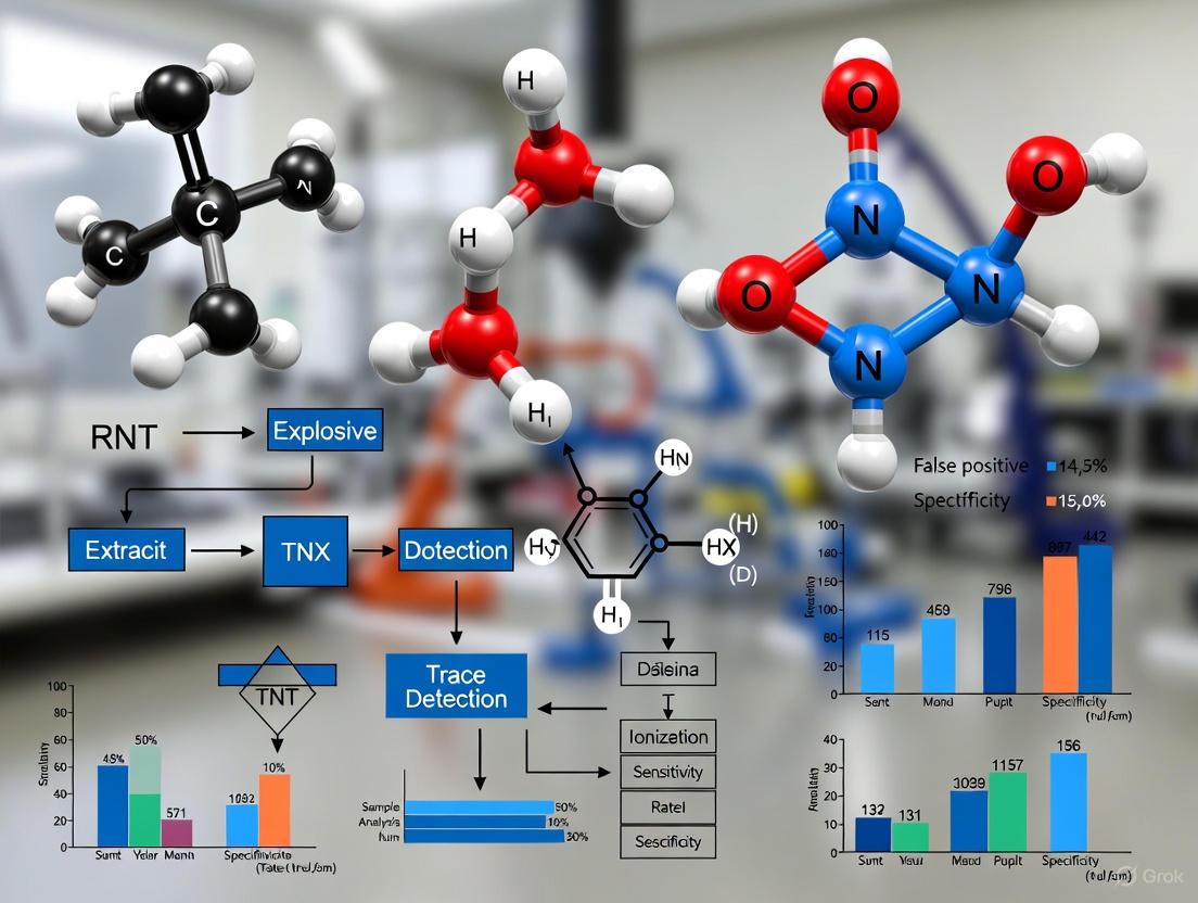
Beyond the False Alarm: Advanced Strategies for Precision in Trace Explosives Detection

Abstract

This article addresses the critical challenge of false positives in trace explosives detection, a key concern for researchers and security professionals developing and deploying these systems. We explore the fundamental causes and impacts of false alarms, from environmental factors to technological limitations. The scope covers established and emerging detection methodologies, including Ion Mobility Spectrometry (IMS), Mass Spectrometry, and fluorescence sensing, alongside targeted optimization techniques such as AI-enabled data analysis and rigorous statistical validation. By providing a comparative analysis of technologies and a framework for performance evaluation, this resource aims to equip professionals with the knowledge to enhance detection accuracy, streamline security operations, and guide future research and development.

Understanding the False Positive Challenge: Sources and Impacts on Security Screening

Technical Support & Troubleshooting Hub

This section provides practical answers to common challenges faced by researchers and scientists working with Explosive Trace Detection (ETD) technologies.

Frequently Asked Questions (FAQs)

Q1: What are the most frequent non-threat sources of false positives in our ETD experiments? A primary source of false positives is cross-talking chemicals present in the testing environment. These include common organic materials such as perfumes, cleaning agents, and fertilizers, which can be misinterpreted by the detector's sensors [1]. Furthermore, incomplete or outdated explosive compound libraries within the system can lead to misidentification of novel or chemically similar substances. Ensuring a clean, controlled sampling procedure and regularly updating threat databases are critical first steps in troubleshooting.

Q2: Our benchtop ETD system is generating a high rate of false alarms, stalling our research throughput. What immediate steps should we take? Begin with a systematic diagnostic of your data inputs and system configuration:

• Verify Data Quality: Confirm that the standard samples and calibration materials are pure, uncontaminated, and properly stored. Poor data quality is a leading cause of erroneous flags [2].
• Review and Update Detection Rules: The detection rules (algorithms or thresholds) in your system may be too rigid. Statically configured systems are a known source of false positives and require consistent evaluation and updating to reflect new knowledge and contexts [2].
• Check for Sensor Contamination: Residue from previous tests can contaminate the sampling interface. Follow the manufacturer's protocol for decontaminating the system.

Q3: How can we future-proof our research against evolving explosive compounds that challenge traditional detection methods? The field is moving towards multi-modal detection systems and the integration of Artificial Intelligence (AI) and Machine Learning (ML). Multi-modal systems that combine trace detection with imaging technologies and chemical analysis offer higher accuracy and reliability against a wider range of compounds [3]. Meanwhile, AI-driven algorithms can enhance detection accuracy by learning complex chemical signatures and adapting to new threats in real-time, significantly reducing false positives [4] [3]. Investing in research platforms that support these technologies is key.

Q4: What is the operational impact of a high false positive rate on a research and development pipeline? High false positive rates lead to operational breakdowns and significant resource waste. They bog down compliance and research teams, forcing them to spend time investigating non-threats instead of focusing on genuine experimental results or novel threats [2]. This not only creates inefficiencies but also delays project timelines and increases operational costs. In a security context, it can also lead to strained customer relationships and a loss of trust in the technology [2].

Quantitative Data: ETD Market and Technology

The following tables summarize key quantitative data and technological trends relevant to planning and evaluating ETD research.

Table 1: Explosive Trace Detection Market Forecast (2024-2035) This data provides context on market growth, which is driven by the need for more accurate and reliable detection technologies.

Region/Segment	2024 Market Size	2035 Projected Market Size	Compound Annual Growth Rate (CAGR)	Key Growth Driver
Global Market [3]	USD 6.92 Billion	USD 12.96 Billion	6.48%	Escalating global security needs, technological innovation
North America [4]	~USD 750 Million (2024)	~USD 1.3 Billion (2033)	6.8% (till 2033)	Government defense & homeland security spending
Asia Pacific [3]	-	-	- (Fastest growing)	Rapid infrastructure development, increasing air travel

Table 2: Top 5 Technology Trends in Explosive Trace Detection Understanding these trends is crucial for directing research into the most promising areas for reducing false positives.

Trend	Description	Impact on False Positives
AI & Machine Learning Integration [3]	Use of algorithms to identify complex chemical signatures more precisely.	Enhances detection accuracy and reduces false alarms by learning and adapting.
Miniaturization & Portability [3]	Development of compact, handheld ETD devices for flexible deployment.	Enables faster, on-the-go screening but requires robust algorithms to maintain accuracy.
Multi-Modal Detection Systems [3]	Combining trace detection with imaging tech and chemical analysis.	Offers higher accuracy and reliability by cross-verifying threats through multiple methods.
Growing Demand in Transportation [3]	Expansion of ETD deployment in airports, rail, and public transit hubs.	Increases the need for fast, non-intrusive, and highly reliable detection to manage high throughput.
Sustainability & Cost-Effectiveness [3]	Focus on devices with lower energy use and minimal consumables.	Reduces operational costs, allowing for broader adoption and investment in advanced R&D.

Experimental Protocols & Methodologies

This section outlines a detailed methodology for a key experiment cited in the literature: implementing a false-positive tolerant model in a distributed learning environment. This is particularly relevant for researchers developing next-generation AI-driven detection algorithms.

Detailed Protocol: Budget-Based Misconduct Mitigation in Distributed Federated Learning

This protocol is based on a study that addressed model integrity and false positives in a collaborative machine learning setting, which can be directly analogized to a multi-instrument or multi-lab ETD research network [5].

1. Problem Formulation & Hypothesis:

• Objective: To mitigate the impact of adversarial or erroneous models ("model misconduct") in a Distributed Federated Learning (DFL) network without excessive ostracization of benign participants due to false positives.
• Hypothesis: A mitigation system that allows for a "misbehavior budget" will more effectively preserve system performance and sample size compared to a zero-tolerance system.

2. Experimental Workflow: The following diagram illustrates the logical workflow of the experiment, showing the critical decision points for identifying and mitigating potential threats while providing tolerance for false alarms.

3. Key Research Reagent Solutions & Materials: This table details the essential "reagents" or components required to replicate this computational experiment.

Table 3: Essential Materials for Distributed Learning Experiment

Item	Function/Description	Relevance to Experiment
Structured EHR Datasets [5]	The source data (e.g., tabular medical data) used to train and validate the predictive models.	Serves as the standardized "sample" for testing the model's performance and resilience.
Decentralized Blockchain Network [5]	A peer-to-peer network that facilitates transparent and tamper-proof model exchanges between nodes.	Replaces a central server, eliminating single points of failure and providing a verifiable audit trail.
Federated Learning Framework [5]	Software that enables the training of a shared model across decentralized devices holding local data.	The core "instrument" that allows collaborative learning without sharing raw data.
Misconduct Detection Heuristic [5]	A pre-existing algorithm or rule set designed to flag a potentially tampered local model.	Acts as the initial "detection sensor" that triggers the mitigation protocol.
Hyperparameter (γ - Gamma) [5]	The budget penalty term; a tunable variable that determines the severity of the penalty for detected misconduct.	A critical experimental parameter that controls the system's tolerance level.

4. Procedure: 1. Network Setup: Establish a DFL network using a blockchain framework with multiple participating nodes (e.g., 3 or more). 2. Model Initialization: Initialize a global machine learning model (e.g., for a predictive health task) and distribute it to all nodes. 3. Training & Injection Cycle: * Each node trains the model on its local dataset and submits the updated model to the network. * For the experimental group: Periodically inject a tampered (misconducted) model from one or more designated nodes to simulate an attack. 4. Mitigation Execution: * For every model submission, run the Misconduct Detection Heuristic. * If misconduct is detected, check the node's remaining "misbehavior budget." * If the budget is exhausted, quarantine the node (exclude its model from aggregation). * If the budget is not exhausted, apply a penalty (γ) to the budget and still allow the model to be included in the aggregation. 5. Aggregation & Iteration: Aggregate the models from non-quarantined nodes to update the global model. Repeat the cycle until model convergence. 6. Control & Ablation: Run a control group with no misconduct and an ablation group that uses a mitigation system with zero tolerance (no budget) to benchmark performance.

5. Performance Metrics:

• Primary Metric: Area Under the Receiver Operating Characteristic Curve (AUC) of the final global model. Compare the mitigated model's AUC against the baseline (no mitigation) and the ablation (zero-tolerance) model [5].
• Secondary Metric: Overhead time required for the mitigation process, which should be negligible (e.g., <12 milliseconds) to be practical [5].

Troubleshooting Guide: FAQs on False Positives

FAQ 1: What are the most common sources of environmental interference causing false positives? Environmental interference stems from chemical compounds in common household and personal items that can be misidentified as explosives by detection systems. Complex mixtures from products like skin lotions, sunscreens, fragrances, and hair products can produce overlapping signals with threat compounds in both Ion Mobility Spectrometry (IMS) and Mass Spectrometry (MS), leading to false alarms [6]. These interferents compete for charge during ionization, potentially suppressing the analyte signal or creating a false threat signature.

FAQ 2: How do substrate materials affect trace explosive sampling and detection? The surface from which a sample is collected—the substrate—significantly impacts sampling efficiency. Porous, rough, or contaminated surfaces can trap explosive particles, making them difficult to recover with a standard swab [7]. Furthermore, chemical interactions between the explosive residue and the substrate material can alter the sample's composition or reduce its availability for analysis, thereby lowering the probability of detection and potentially leading to false negatives or inconsistent results [7].

FAQ 3: What are the key limitations of current detection reagents and sensing materials? Many fluorescent sensing materials, while highly sensitive, can be affected by environmental factors such as UV light, leading to photodegradation and signal decay over time [8]. Their preparation processes are often complex, and their performance can be influenced by the specific substrate preparation method (e.g., spin-coating, acid corrosion, baking) [8]. The need for rigorous stability testing and optimization of the material's immobilization process is a critical limitation for field deployment.

FAQ 4: How can I validate that a positive signal is a true positive and not an instrument error? Validation requires a method that provides high specificity. Techniques like Gas Chromatography-Mass Spectrometry (GC-MS) separate compounds before analysis, providing a distinct "molecular fingerprint" that can confirm the presence of a specific explosive and rule out interferents [9] [10]. For spectroscopic methods, applying machine learning algorithms trained to recognize the target compound's signature amidst background noise can significantly improve confidence in the result [11].

FAQ 5: What emerging technologies can help overcome false positive challenges? Several advanced technologies show great promise:

• Surface-Enhanced Raman Spectroscopy (SERS): Offers a highly sensitive and specific molecular fingerprint, capable of detecting trace amounts of explosives [9] [12].
• Artificial Intelligence and Machine Learning (AI/ML): These systems can be trained to distinguish target explosives from complex background interferents with high probability of detection (PD) and low probability of false alarm (PFA), and they can update threat libraries rapidly [11].
• Ambient Ionization Mass Spectrometry (AIMS): Allows for direct analysis of samples with minimal preparation, enabling rapid, high-throughput examination ideal for field applications [9].

Table 1: Comparison of Explosive Trace Detection Techniques and False Positive Challenges

Detection Technique	Target Analytes	Key Sources of Interference/Limitations	Typical LOD
Ion Mobility Spectrometry (IMS)	Organic explosives [10]	Personal care products (lotions, sunscreens, fragrances) [6]	pg–ng [10]
Mass Spectrometry (MS)	All (depending on ionization) [10]	Chemical noise in complex samples; overlapping nominal masses [6]	pg–ng [10]
Fluorescence Sensing	Nitroaromatics (e.g., TNT) [8]	Sensor photodegradation; complex film preparation [8]	0.03 ng/μL (for TNT acetone solution) [8]
Raman/SERS	Raman-active explosives [9] [10]	Background fluorescence; requires noble metal substrates [9]	μg/ng (SERS) [10]
Gas Chromatography-MS (GC-MS)	Volatile and semi-volatile explosives [9]	Lengthy analysis time; not ideal for non-volatile compounds [6]	High sensitivity (precise LOD varies) [9]

Table 2: Experimental Protocol for Characterizing Fluorescent Sensor Stability

This protocol is adapted from research on TNT-detecting fluorescent films [8].

Step	Procedure	Purpose/Function
1. Film Preparation	Prepare fluorescent films (F1-F5) with varying processes: standard spin-coating (F1), substrate etching (F2, F3), and antioxidant addition (F4, F5).	To evaluate how different fabrication methods impact sensor stability and performance.
2. Photostability Testing	Expose films to UV light and measure fluorescence intensity decay at different time intervals.	To quantify the sensor's resistance to photodegradation, a key limitation.
3. Calculate Decay Rate	Use the formula: Fluorescence Intensity Decay Rate = ((I0 - It)/I0) where (I0) is initial intensity and (I_t) is intensity at time t.	To objectively compare the stability and service life of different film formulations.

The Scientist's Toolkit: Research Reagent Solutions

Key Materials for Trace Explosives Detection Research

Item	Function in Research
Fluorescent Sensing Material (e.g., LPCMP3)	Serves as the active element in a sensor; undergoes fluorescence quenching upon interaction with nitroaromatic explosives like TNT via photoinduced electron transfer (PET) [8].
High-Purity Analytical Standards	Essential for calibrating instruments like GC-MS and LC-MS; used to confirm the identity and quantify trace levels of explosives, ensuring accurate identification against background interferents [10].
Personal Care Product Mixtures	Used as complex sample matrices to test for false positive responses and evaluate the selectivity and robustness of a detection method against common environmental interferents [6].
Noble Metal Substrates (for SERS)	Nanostructured surfaces (e.g., of gold or silver) that dramatically enhance the Raman signal of target molecules, enabling single-molecule level detection sensitivity for explosives [9] [12].
Machine Learning Training Datasets	Curated collections of spectrographic data (e.g., from Raman spectroscopy) for known explosives and interferents; used to "teach" AI/ML algorithms to accurately classify threats and reduce false alarms [11].

Experimental Validation and Technology Comparison

Diagram: Workflow for AI-Enhanced Explosive Detection Validation

Diagram: Technology Comparison for False Positive Mitigation

Frequently Asked Questions (FAQs)

Q1: What defines a false alarm in the context of trace explosives detection? A false alarm, or false positive, occurs when a detection system incorrectly identifies a benign substance or activity as a potential explosive threat [13]. In practice, this means an alert is triggered, and resources are deployed to investigate, but no actual threat is present. It is crucial to distinguish these from false negatives, where an actual explosive threat is not detected by the system [14].

Q2: What are the primary real-world costs associated with false alarms? The costs are multi-faceted and extend beyond simple financial metrics [13]:

• Resource Drain: Each false alarm wastes the time of highly trained personnel (e.g., Transportation Security Officers, scientists) on investigations of clean samples. This includes the costs of dispatched personnel, call takers, and equipment depreciation [13].
• Alert Fatigue: A constant flood of false alarms leads to analyst and operator burnout, a state of desensitization where there is a risk of missing or ignoring genuine incidents. Research indicates that security teams can spend an estimated one-third of their workday on incidents that are not real threats [15] [16].
• Throughput Degradation: False alarms and system downtime directly slow the screening process. During an outage or recovery, a backlog of samples builds up, increasing the Mean Time to Respond (MTTR) and creating significant delays for passengers or samples waiting to be processed [17] [18].
• Eroded Confidence: Persistent false positives can pollute compliance reports and erode executive and public confidence in the security system's effectiveness [17].

Q3: What are the common root causes of false positives in detection systems? Common causes include [13]:

• Oversensitive Sensors: Sensors configured without adequate filtering for non-threat environmental noise (e.g., pets, cleaning equipment, environmental vibrations).
• System Misconfiguration: Poorly tuned detection rules, outdated threat libraries, or incorrect sensitivity settings.
• Environmental Factors: Poor sensor placement (e.g., next to heating ducts or fans), poor wiring, or a lack of system maintenance.
• Human Error: Users failing to properly arm/disarm systems or input correct security codes.
• Technology Limitations: Reliance on outdated "Sensing 1.0" technologies that cannot learn or distinguish between normal and abnormal patterns with high fidelity [13].

Q4: Our detection pipeline is experiencing performance degradation and high latency. How can we model this? You can model a pipeline's health using concepts of availability and capacity. The total disruption time (A) from an outage of duration (T) can be modeled algebraically if your system has an over-provisioning factor (N), which is the ratio of your system's peak processing capacity to its average data arrival rate (R) [18].

The formulas are:

• Recovery Time, P = T / (N-1)
• Total Disruption Time, A = T + P = T × [N / (N-1)]

This model shows that without over-provisioning (N=1), the system never recovers from backlog. The benefit of over-provisioning has diminishing returns; increasing N from 2 to 3 has a significant impact, but gains become minimal beyond N=6 [18].

Q5: What are the key strategies for reducing false alarm rates? A multi-pronged approach is most effective:

• Advanced Sensing Technology: Transition to "Sensing 2.0" technologies, such as WiFi sensing or AI-enabled mass spectrometry, that use intelligent algorithms to learn and filter out common false alarm sources [13] [19].
• Contextual Enrichment and Correlation: Use systems that correlate data from multiple sources (e.g., endpoint, network, vapor) to provide context, rather than relying on isolated signals [20].
• Regular Tuning and Maintenance: Clearly define detection use cases, create runbooks for alerts, and regularly test, tune, and update detection rules and system thresholds. This includes maintaining hardware and replacing degraded components [13] [15].
• Implement a Feedback Loop: Establish a process to classify all alerts (e.g., as false positive or true positive). Use this data to feed back into the system, making the threat intelligence smarter over time [14] [16].

Troubleshooting Guides

Guide: Diagnosing and Resolving a High Rate of False Positives

This guide helps researchers and technicians systematically identify the source of false positives in their trace detection systems.

Step	Action	Expected Outcome	Underlying Principle
1. Identify Source	Review alert logs to determine if the detection is from a specific sensor, a particular detection rule (e.g., for a specific explosive compound), or an environmental zone.	The alert source is pinpointed (e.g., "Vapor Sampler A," "IMS library entry for Compound X").	Accurate diagnosis requires understanding the detection source, similar to identifying EDR vs. Antivirus alerts in cybersecurity [14].
2. Classify the Alert	Manually verify the sample that triggered the alarm. Classify the alert as a False Positive (system error), True Positive Benign (correct detection of a non-threat substance, like a legal solvent), or True Positive (actual threat).	A clear classification that informs the next step.	Classifying alerts helps train your system and reduces false positives over time. It also differentiates system error from correct identification of benign substances [14] [15].
3. Implement Short-Term Workaround	If the false positives are overwhelming, create a temporary exception or exclusion for the specific substance or sensor. Caution: This lowers your protection level and should be a temporary fix [14].	A reduction in noise, allowing operators to focus.	This is a tactical mitigation to maintain operational throughput while a root cause is found [14].
4. Root Cause Analysis & Long-Term Fix	Investigate the root cause based on the source and classification.	A permanent resolution, such as a retuned sensor, an updated threat library, or a moved sensor.	Addressing the root cause (e.g., misconfiguration, poor placement) prevents recurrence [13] [15].

Detailed Root Cause Analysis (Step 4):

• If the cause is a misconfigured sensor: Adjust the sensitivity thresholds or apply filtering algorithms to ignore common non-threat particulates [13].
• If the cause is an outdated threat library: Update the device's explosive compound library to better distinguish between threat and non-threat substances [19].
• If the cause is environmental: Relocate the sensor away from air vents, vibrations, or areas with high human traffic that is not a security boundary [13].
• If the cause is system degradation: Check for hardware issues like poor wiring, low batteries, or need for component replacement [13].

Guide: Addressing Performance Degradation and Latency in Detection Pipelines

This guide addresses slowdowns in automated sample processing and analysis pipelines.

Symptom	Potential Cause	Diagnostic Action	Resolution
Consistently high processing latency across all samples.	An overall throughput degradation in one or more pipeline components (e.g., a spectrometry runtime or database is performing sub-optimally).	Check health metrics of all pipeline components (CPU, memory, I/O). Identify the component with the highest resource utilization or error rate.	Scale up the affected component (e.g., add more compute resources). If it's a software issue, a restart or patch may be required [18].
A growing backlog of samples waiting to be analyzed; system is falling behind.	Insufficient capacity (Low N) to handle the average arrival rate R of samples, or a complete outage from which the system is struggling to recover.	1. Calculate your pipeline's over-provisioning factor N. 2. Check logs for recent outages.	Increase the pipeline's peak processing capacity (N*R). The algebraic model P = T/(N-1) can help calculate the required N to achieve a desired recovery time P [18].
Delays and latency spikes occurring in regular, predictable waves.	"Tsunami traffic" or scheduled bulk data ingestion, overwhelming the pipeline's standard capacity [18].	Analyze traffic patterns to confirm peaks align with specific events or batch processes.	Implement auto-scaling rules to proactively add capacity before predicted traffic peaks. Alternatively, smooth out data ingestion schedules [18].

Table 1: Quantified Impact of False Alarms and System Downtime

Metric	Quantitative Finding	Source / Context
Prevalence of False Alarms	94-98% of all alarm calls in public safety; up to 63% of daily alerts in SOCs are false positives or low-priority [13] [15].	Public safety & cybersecurity contexts, demonstrating universality of the problem.
Productivity Loss	Security analysts spend an estimated one-third of their workday on non-actionable incidents [15].	Based on a survey of 1,000 Security Operations Center (SOC) members.
Annual Cost to Services	Estimated $1.8 billion annual cost to emergency services in the U.S. [13].	Study by the Center for Problem-Oriented Policing.
Pipeline Availability Impact	A pipeline with 12 components, each with 99.99% availability, has a combined availability of only 99.88% (~10.5 hours downtime/year) [18].	Analytical model for distributed systems.
Recovery Time Model	Total disruption time A = T × [N / (N-1)], where T is outage duration and N is over-provisioning factor [18].	Algebraic model for pipeline recovery.
Clinically Actionable Alerts	In one emergency department study, only 1% of alarms from equipment like electrocardiograms were clinically actionable [13].	Healthcare context, showing false alarms are a cross-industry issue.

Experimental Protocols & Methodologies

Protocol: Validating Reductions in False Positives for a Novel ETD Technology

Objective: To empirically demonstrate that a new Explosives Trace Detection (ETD) technology or a tuning adjustment significantly reduces the false positive rate (FPR) without compromising the true positive detection rate.

Materials:

• The ETD system under test (e.g., Next-Gen Mass Spectrometry ETD, Vapor Detection wand).
• A validated library of explosive compounds.
• Test swabs and sample containers.
• A set of controlled, benign substances that are known to historically trigger false alarms (e.g., common fertilizers, legal solvents, personal care products, pharmaceuticals).
• A set of trace samples of target explosive materials.

Methodology:

• Baseline Establishment: Using the current/old technology or configuration, process 1000 samples. The sample set should be a blind mix of 5% true explosive traces and 95% benign substances, including the known interferents.
• Test Run: Using the new technology or tuning, process the same 1000-sample set under identical environmental and operational conditions.
• Data Collection: For both runs, record for each sample:
  • Alert Triggered (Yes/No)
  • Substance Identified
  • Ground Truth (Whether it was an explosive or benign)
• Analysis: Calculate the following metrics for both the baseline and test runs:
  • False Positive Rate (FPR): (Number of benign samples that triggered an alert) / (Total number of benign samples)
  • True Positive Rate (TPR) / Sensitivity: (Number of explosive samples correctly identified) / (Total number of explosive samples)
  • Throughput: Average number of samples processed per hour.

Validation: A successful experiment will show a statistically significant reduction in FPR in the test run compared to the baseline, while maintaining or improving the TPR and throughput.

Workflow: System Validation for False Positive Reduction

The following workflow diagrams the experimental and operational process for implementing and validating a false positive reduction strategy, from initial detection to system refinement.

The Scientist's Toolkit: Research Reagent Solutions

Table 2: Essential Materials for Explosives Trace Detection Research

Item / Solution	Function in Research & Development
Next-Gen Mass Spectrometry ETD	Provides high-sensitivity and high-resolution detection of explosive residues. Its expandable library allows for identifying novel explosives, directly reducing false negatives against emerging threats [19].
Explosives Vapor Detection (EVD) Samplers	Enables non-contact sampling by liberating and analyzing particulate vapors. Critical for developing faster, less intrusive screening methods and understanding vapor signatures [19].
Ion Mobility Spectrometry (IMS)	The core technology in many deployed ETDs. It ionizes sample molecules and identifies them based on their drift speed in a carrier gas. Research focuses on improving its sensitivity and specificity [19].
Channel State Information (CSI) Filters	Used in WiFi sensing and other advanced detection methods. Raw CSI data is pre-filtered to rule out non-human movements (e.g., pets), forming the first stage of false alarm reduction in "Sensing 2.0" systems [13].
AI & Machine Learning Algorithms	Applied to filtered sensor data for higher-level processing. These algorithms learn to distinguish normal from abnormal patterns, analyze breathing patterns, or identify repetitive movements, drastically reducing false positives in complex environments [13] [20].
Customizable Detection Rules	Allow researchers to fine-tune detection thresholds and logic based on specific operational environments and threat models, which is key to managing the false positive rate [20].

FAQs: Navigating Detection Specificity in HME Analysis

FAQ 1: What are the primary factors contributing to false positives when detecting inorganic HMEs? False positives in inorganic HME detection primarily arise from matrix effects and chemical interferences. Complex samples, such as personal care products (e.g., skin lotions, sunscreens, and fragrances), can produce overlapping mobility peaks in Ion Mobility Spectrometry (IMS) and isobaric interferences in mass spectrometry (MS) operated in nominal mass mode, leading to false alarms for explosive compounds [6]. The vast array of potential organic fuels in fuel-oxidizer mixtures also makes it difficult to differentiate target analytes from environmental background clutter [21].

FAQ 2: Why do many standard field detection methods struggle with HMEs based on grocery powders and hydrogen peroxide? Standard methods like portable Raman or FT-IR spectroscopy struggle with these HMEs because the IR spectra of the oxidized grocery powders (e.g., coffee, tea, spices) show only minor and non-characteristic changes compared to their untreated states [22]. The explosive mixture does not produce strong, unique vibrational fingerprints that are easily distinguishable from the underlying organic plant material, making direct identification via these techniques challenging without advanced data analysis [22].

FAQ 3: How can researchers improve the specificity of trace explosive detection for complex mixtures? Improving specificity involves a multi-faceted approach:

• Employ Data Fusion Techniques: Integrating multiple analytical techniques, such as combining Ion Mobility Spectrometry with Mass Spectrometry (IMMS), provides two orthogonal data dimensions (drift time and m/z) to separate target explosives from chemical noise [6].
• Utilize Advanced Data Processing: Applying similarity measures and machine learning algorithms to time-series sensor data or complex spectra can enhance classification. For example, integrating Spearman correlation coefficients and Derivative Dynamic Time Warping (DDTW) distance has been used to effectively classify fluorescence-based detection results [8].
• Target Specific Molecular Markers: For challenging HMEs like H₂O₂-based mixtures, use targeted analytical techniques like GC-MS to identify unique oxidation byproducts. For instance, dimethylparabanic acid (DMPA) is a specific marker for black tea oxidized by hydrogen peroxide [22].

Troubleshooting Guides: Common Experimental Pitfalls and Solutions

Troubleshooting Guide 1: Fluorescence Quenching Sensor Performance

This guide addresses issues when developing fluorescent sensors for nitroaromatic explosives like TNT.

Problem Symptom	Potential Cause	Solution & Verification Protocol
Low or unstable fluorescence signal from the sensing film.	Poor film photostability or degradation of the fluorescent material.	Verify Protocol: Prepare films using different substrate treatments and drying processes [8]. Compare fluorescence intensity decay rates under continuous UV illumination. Films with added antioxidant (e.g., F5 film) and baked at 60°C demonstrate superior stability [8].
Slow response time (>5 seconds) or incomplete recovery (>1 minute).	Sub-optimal film morphology or thick polymer layers hindering analyte diffusion.	Verify Protocol: Ensure fluorescent film is prepared by spin-coating at high rotational speed (e.g., 5000 rpm) to create a thin, uniform layer [8]. Test response to a standard TNT acetone solution (e.g., 0.03 ng/μL). A functional sensor should respond in <5 s and recover in <1 min [8].
Lack of specificity; quenching by common interferents.	Insufficient selectivity of the fluorescent polymer.	Verify Protocol: Conduct selectivity tests with common chemical reagents and potential interferents. A specific sensor should show significant quenching only with nitroaromatic explosives like TNT, not with other benign chemicals [8].

Troubleshooting Guide 2: Ion and Mass Spectrometry Analysis

This guide tackles challenges in detecting trace explosives in complex matrices using spectrometric techniques.

Problem Symptom	Potential Cause	Solution & Verification Protocol
High false positive rate in complex samples.	Insufficient resolving power leading to overlapping peaks from sample matrix.	Verify Protocol: For IMS, this is a known limitation (Rp 20-40). For MS, operate the instrument at its highest possible resolving power. For laboratory-based analysis, use LC- or GC-MS to separate analytes from interferents before mass analysis [6].
Signal suppression or decreased sensitivity for the target analyte.	Matrix effects where interferents compete for charge during ionization.	Verify Protocol: Use a standard addition method to quantify suppression. Employ sample pre-separation or clean-up steps to reduce matrix complexity. In ambient ionization, optimize the ion source to favor the target analyte [6].
Inability to detect inorganic oxidizers (e.g., nitrates, chlorates).	Inefficient ionization of target inorganic species with the selected method.	Verify Protocol: Implement alternative ionization schemes or pre-separation techniques designed for inorganics, such as capillary electrophoresis or chemical conversion methods that transform the oxidizer into a more easily detectable species [21] [23].

Quantitative Data: Performance Metrics for Explosives Detection

The following tables summarize key performance data from recent research on trace explosive detection to aid in method selection and benchmarking.

Table 1: Performance of Fluorescence-Based Trace Explosives Detection

Data sourced from fluorescence sensing research for nitroaromatic compounds [8].

Detection Parameter	Reported Performance Metric
Target Analyte	2,4,6-trinitrotoluene (TNT) in acetone solution
Limit of Detection (LOD)	0.03 ng/μL
Response Time	< 5 seconds
Recovery Time	< 1 minute
Key Material	LPCMP3 fluorescent polymer
Classification Method	Spearman correlation coefficient & DDTW distance

Table 2: Comparative False Positive Analysis for Spectrometric Techniques

Data based on analysis of 18 common household products [6].

Analytical Technique	Operating Mode	False Positive Occurrence	Primary Challenge
Ion Mobility Spectrometry (IMS)	Standalone	Common in complex samples	Overlapping mobility peaks
Mass Spectrometry (MS)	Nominal Mass (Unit Resolution)	As common as in IMS	Isobaric interferences from chemical noise
Ion Mobility-Mass Spectrometry (IMMS)	2D Mobility-Mass	Significantly reduced	Provides orthogonal separation (drift time & m/z)

Table 3: Molecular Markers for H₂O₂-Grocery Powder HMEs

Data for identifying post-blast residues or unexploded mixtures via GC-MS [22].

Grocery Powder	Key Molecular Marker(s)	Notes on Marker Stability
Black Tea	Dimethylparabanic Acid (DMPA)	Best for fresh samples; concentration decreases over extended periods (e.g., 1 week).
Coffee	Specific oxidation products of triglycerides & fatty acids (e.g., from oleic acid).	Requires monitoring of multiple compounds due to complex composition.
Paprika & Turmeric	Oxidation products of unsaturated fatty acids and pigments (curcuminoids).	Markers are stable, but their profile changes over time as oxidation progresses.

Experimental Protocols: Detailed Methodologies for Key Experiments

Protocol 1: Fabrication and Testing of a Fluorescent Sensor for TNT

Objective: To create a functional fluorescent thin film sensor for the trace detection of nitroaromatic explosives and characterize its performance [8].

Materials:

• Fluorescent Material: LPCMP3 polymer.
• Solvent: Tetrahydrofuran (THF).
• Substrate: Quartz wafer.
• Equipment: Micropipette, spin-coater (e.g., TC-218), oven.

Methodology:

• Solution Preparation: Weigh 10 mg of LPCMP3 solid and dissolve in 1 mL of THF. Protect from light and let stand for 30 minutes until fully dissolved to obtain a stock solution. Dilute to a working concentration of 0.5 mg/mL.
• Film Fabrication: Using a micropipette, deposit 20 μL of the working solution onto the center of a clean quartz wafer. Immediately spin-coat the wafer at 5000 rpm for 60 seconds to form a uniform thin film.
• Film Post-treatment: For enhanced stability, bake the spin-coated film in an oven at 60°C for 15 minutes.
• Performance Testing:
  • Quenching Test: Expose the film to vapors or solutions containing the target analyte (e.g., TNT in acetone at varying concentrations) under UV illumination (max absorption ~400 nm).
  • Data Acquisition: Monitor the fluorescence emission (max emission ~537 nm) over time to record the quenching response and subsequent recovery.
  • Data Analysis: Calculate the fluorescence intensity decay rate. Use time-series similarity measures (e.g., Spearman correlation coefficient, DDTW) to classify the response.

Protocol 2: GC-MS Analysis of H₂O₂-Grocery Powder HME Residues

Objective: To identify unique molecular markers in homemade explosives composed of hydrogen peroxide and common grocery powders [22].

Materials:

• Samples: Ground roasted coffee, black tea, sweet paprika, turmeric, and concentrated hydrogen peroxide (50-60% w/w).
• Solvents: Methanol, high-purity for extraction.
• Equipment: GC-MS system, standard sample preparation tools.

Methodology:

• Sample Preparation: Mix the selected grocery powder with concentrated H₂O₂ to form a paste. For kinetic studies, allow the mixture to react for varying time intervals (e.g., 1, 5, 60 minutes, 1 week).
• Extraction: At each time point, stop the reaction by diluting and extracting the mixture with methanol.
• GC-MS Analysis:
  • Chromatography: Inject the methanolic extract into the GC-MS system. Use a standard non-polar to mid-polar capillary column with a programmed temperature ramp to separate the complex mixture of compounds.
  • Mass Spectrometry: Operate the MS in electron impact (EI) mode. Scan a mass range suitable for small organic molecules (e.g., m/z 40-500).
• Data Interpretation:
  • Compare chromatograms of untreated grocery powders with those of H₂O₂-treated samples to identify new peaks corresponding to oxidation products.
  • Identify these marker compounds (e.g., Dimethylparabanic Acid in tea) by comparing their mass spectra with libraries and authentic standards when available.
  • Monitor the kinetics of marker formation and degradation to assess the age of the explosive mixture.

Research Reagent Solutions: Essential Materials for HME Detection Research

A curated list of key reagents and materials used in advanced explosives detection research, as cited in the literature.

Reagent/Material	Function/Application in Research
LPCMP3 Polymer	Fluorescent sensing material for nitroaromatic explosives (e.g., TNT) via photoinduced electron transfer (PET) [8].
Tetrahydrofuran (THF)	Solvent for dissolving and processing fluorescent polymers for thin-film sensor fabrication [8].
Hydrogen Peroxide (50-60% w/w)	Key oxidizer precursor in powerful HMEs based on grocery powders (e.g., coffee, tea, flour) [22].
Powdered Groceries (Coffee, Tea, Spices)	Act as organic fuels in H₂O₂-based HMEs; source of specific molecular markers for forensic analysis via GC-MS [22].
Antioxidant 891	Additive used in fluorescent film preparation to enhance photostability and operational lifetime [8].

Detection Workflows and Chemical Pathways

Multimodal Detection Workflow for Trace Explosives

H₂O₂-Grocery Powder HME Marker Formation

Detection Technologies in Practice: From Established Workhorses to Emerging Sensing Platforms

IMS Frequently Asked Questions

What are the fundamental principles behind IMS separation?

Ion Mobility Spectrometry separates ionized molecules in the gas phase based on their mobility under an electric field. Ions are driven through a buffer gas (like air) in a drift tube by an electric field. Larger ions collide with gas molecules more frequently and are slowed down, resulting in longer drift times. The core measurement is the ion's mobility (K), which can be normalized to standard conditions (reduced mobility, K0) and often converted into a collision cross section (CCS), a measure of the ion's gas-phase size [24] [25] [26].

Why does IMS sometimes produce false positive alarms?

False positives primarily occur due to limited resolution and interfering substances. Key reasons include:

• Co-eluting Interferents: Environmental contaminants or chemical interferents with similar drift times to the target analyte can trigger false alarms. Their signal can overlap with the target's detection window, especially in complex samples like swabs from dirty surfaces [27] [25].
• Limited Resolution: The physical length of the drift tube determines the resolution. Compact instruments with shorter tubes have a lower ability to distinguish between ions of very similar mass and size. While deflectors can improve resolution, they are difficult to implement in portable devices [25].
• Environmental Factors: Changes in temperature and humidity can affect measurement stability and contribute to variance in results, potentially leading to false alarms [28].

How can I improve the specificity and reliability of my IMS measurements?

• Optimize Instrument Configuration: Adjusting parameters like desorber temperature, drift tube temperature, and reactant ion chemistry (dopants) can enhance selectivity for specific compound classes [27].
• Employ Multi-Dimensional Separation: Coupling IMS with a preceding separation technique like Gas Chromatography (GC) or Liquid Chromatography (LC) can separate complex mixtures before IMS analysis, reducing interferents [24] [26].
• Use Characterized Calibrants: For techniques like TWIMS, using calibrant ions with well-characterized CCS values is essential for accurate identification [24].
• Characterize Background: For field applications, systematically analyzing the environmental background at the specific screening location helps identify common interferents and set appropriate alarm thresholds [27].

Troubleshooting Common IMS Experimental Issues

Problem: High Variance in Replicate Measurements During Trace Detection

• Potential Cause: Instability during initial device operation or sensitivity to operational conditions.
• Solution: Allow the instrument to stabilize through extended use. One study found that variance fluctuations in one device stabilized only after a significant number of consecutive operations. Ensure consistent sample introduction and swab placement [28].

Problem: Overlapping Peaks for Target Analytes and Interferents

• Potential Cause: The environmental background contains compounds with mobilities similar to your target, a common challenge in real-world screening.
• Solution: Implement a Receiver Operating Characteristic (ROC) curve methodology to quantify the trade-off between sensitivity and specificity. This helps determine the optimal alarm threshold that maximizes true positive rate while minimizing false positives for your specific environment [27].

Problem: Low Sensitivity or Signal Intensity

• Potential Cause: Inlet or desorber temperature is incorrect, or the instrument is overloaded with sample.
• Solution: Verify and adjust desorber and inlet temperatures according to manufacturer guidelines for your target analytes. Pay precise attention to sample presentation; overloading the instrument can cause serious malfunctions and should be avoided [27] [25].

Quantitative Performance Data for IMS-Based Detection

The following tables summarize key performance metrics from recent studies to aid in experimental design and expectation setting.

Table 1: Key Specifications of Two Commercial IMS-Based Explosive Trace Detectors

Device Specification	Product A	Product B
Ionization Technique	Dielectric Barrier Discharge (DBD)	Impulsed Corona Discharge (ICD)
Operational Stability	Stable measurements throughout consecutive operations	Variance fluctuations that stabilized after extended use
Typical Use Case	Long-term laboratory-based operation	Compact, portable, or field-deployable systems

Table 2: Detection Performance for Target Compounds Against Environmental Interferents [27]

Performance Metric	Details	Experimental Findings
Sensitivity (TPR)	True Positive Rate for fentanyl and related compounds	Single to tens of nanograms with ≥90% TPR achievable
Specificity (1-FPR)	False Positive Rate against environmental background	≤2% FPR achievable for most target compounds
Key Challenge	Areas of high interference in reduced mobility spectrum	Some mobility regions have elevated FPR, effectively reducing sensitivity

Experimental Protocols for Key Applications

Protocol: Evaluating IMS Performance Using ROC Curves [27]

This protocol is designed to assess the discriminative potential of an IMS instrument in a specific screening environment, such as vehicle or package screening.

• Background Characterization: Collect a large number (e.g., thousands) of environmental background samples from the actual operational environment using standard swipe sampling methods (e.g., Nomex wipes).
• True Positive Samples: In a laboratory setting, prepare known masses of target analytes (e.g., 1, 10, 100 μg/mL in methanol) and deposit them onto collection wipes. Conduct 10-30 replicates per mass loading.
• Data Collection: Analyze all background and true positive samples using the IMS instrument under evaluation. Archive all data files.
• Data Processing: For each target compound, identify its characteristic detection window (drift time or reduced mobility value).
• ROC Analysis: For a range of alarm thresholds, calculate the True Positive Rate (TPR = number of true positive alarms / total true positive samples) and False Positive Rate (FPR = number of false alarms from background / total background samples). Plot TPR against FPR to generate the ROC curve.
• Threshold Selection: Use the ROC curve to select an alarm threshold that meets the required operational balance between sensitivity (high TPR) and specificity (low FPR).

Protocol: Assessing Measurement Uncertainty in IMS-ETDs [28]

This statistical method helps quantify the reliability of consecutive measurements.

• Sample Preparation: Apply a consistent mass of target analyte (e.g., TNT at the 5 ng detection limit) to swabs at the specified location.
• Consecutive Operation: Perform repeated measurements in set intervals (e.g., 20, 40, 60, 80 operations). For each interval, perform a total number of measurements that is a common multiple (e.g., 240).
• Cleaning Cycle: After completing each interval cycle, activate the instrument's built-in cleaning function for a fixed duration (e.g., 2 minutes).
• Data Recording: Record the quantitative measurement value for each operation.
• Uncertainty Calculation: Perform a Type A evaluation of measurement uncertainty. Calculate the standard uncertainty (uA = sample standard deviation / √n) and the expanded uncertainty (U = k * uA, where k is a coverage factor, typically 2 for 95% confidence).

The Scientist's Toolkit: Key Research Reagent Solutions

Table 3: Essential Materials for IMS Experiments in Trace Detection

Item	Function / Application	Example Use Case
Isobutyramide	Reactant ion chemistry and calibrant (K0 = 1.495 cm²/Vs)	Used in positive ion detection mode for narcotics and explosives in specific instrument configurations [27].
Nicotinamide	Reactant ion chemistry and calibrant (K0 = 1.86 cm²/Vs)	An alternative chemistry for positive ion mode, often used for drug detection [27].
Meta-Aramid Wipes (Nomex)	Wipe-based sample collection from surfaces	Standardized swabbing of target locations (e.g., door handles, steering wheels) for field sampling [27].
Calibrant Ions with Known CCS	Reference compounds for system calibration	Essential for calculating CCS values of unknown analytes in techniques like TWIMS [24].
Acetone, Chlorinated Solvents	Dopant materials for ionization selectivity	Added to drift gas to enhance sensitivity and selectivity for specific compound classes (e.g., acetone for chemical warfare agents) [26].

Logical Workflow for IMS Method Development

The following diagram illustrates a systematic approach to developing and troubleshooting an IMS method for trace detection, incorporating strategies to mitigate false positives.

The Rise of Mass Spectrometry and Raman Spectroscopy for Enhanced Molecular Fingerprinting

The detection of trace explosives in complex samples presents a significant challenge for security and forensic sciences. False positive responses can lead to unnecessary alarms, operational delays, and ultimately undermine the reliability of screening systems. Research has demonstrated that neither Ion Mobility Spectrometry (IMS) nor Mass Spectrometry (MS) alone can provide 100% assurance against false responses when analyzing complex mixtures found in common household products and personal care items [6] [29]. The fundamental issue stems from the vast array of compounds in these products that can share identical mass-to-charge ratios or mobility drift times with target explosive compounds, leading to incorrect identifications [29].

This technical support center provides troubleshooting guidance and methodological protocols for researchers utilizing Mass Spectrometry and Raman Spectroscopy to overcome these challenges. By implementing proper instrumentation practices, calibration procedures, and data analysis techniques, scientists can significantly reduce false positive rates and enhance the reliability of molecular fingerprinting for trace explosives detection.

Mass Spectrometry Troubleshooting Guide

Common Issues and Solutions for Mass Spectrometry

Q: What are the primary causes of false positives in mass spectrometry analysis of trace explosives?

A: False positives in MS analysis primarily occur due to chemical interferents in complex samples that share the same mass-to-charge ratios as target explosive compounds. Common household products, personal care items, and food ingredients contain compounds that can produce mass responses identical to explosive analytes [6]. When MS is operated in nominal mass mode (similar to field instruments), false positive responses are as common as in ion mobility spectrometers [6]. Sample separation before mass analysis is typically required to reduce these false responses [6].

Q: How can I troubleshoot sensitivity loss and potential leaks in my mass spectrometer?

A: Follow this systematic approach to identify and resolve sensitivity issues:

• Check for gas leaks using a leak detector, particularly after installing new gas cylinders [30]
• Inspect gas filters and tighten if loose [30]
• Examine shutoff valves as moving parts are prone to leaking [30]
• Verify EPC connections where gas enters the system [30]
• Check weldment lines and column connectors - retighten if leaking, replace if cracked [30]

Q: What should I do when my mass spectrometer shows no peaks in the data?

A: The absence of peaks typically indicates either detector issues or problems with sample delivery:

• Verify auto-sampler and syringe function to ensure proper sample introduction [30]
• Check sample preparation to confirm proper formulation [30]
• Inspect the column for cracks which would prevent material from reaching the detector [30]
• Confirm detector operation including flame status and proper gas flow [30]

Comparative Performance of Detection Techniques

Table 1: Comparison of Analytical Techniques for Trace Explosives Detection

Technique	False Positive Rate	Resolving Power	Analysis Time	Key Limitations
Mass Spectrometry (MS)	Similar to IMS in nominal mass mode [6]	4,000-40,000 [6]	Varies with method	Chemical interferents from complex samples [6]
Ion Mobility Spectrometry (IMS)	Low, but significant with complex mixtures [6]	20-40 [6]	<6 seconds [6]	Mobility overlaps from personal care products [6]
MS-IMS Combined	No false responses when both dimensions used [6]	Combined power of both techniques	Longer than IMS alone	More complex instrumentation [6]
Raman Spectroscopy	Low with proper calibration	Spectral resolution dependent on instrument	Seconds to minutes	Fluorescence interference [31]

Experimental Protocol for Reducing False Positives in MS

Materials and Reagents:

• Calibration standards specific to target explosives
• High-purity solvents (HPLC grade)
• Personal care product mixtures for interference testing
• Gas leak detector
• Reference explosive compounds

Procedure:

• System Calibration

  • Perform daily calibration using certified reference materials
  • Verify mass accuracy across expected range
  • Confirm resolution meets manufacturer specifications

• Sample Preparation

  • Implement solid-phase extraction to remove interferents
  • Use internal standards to correct for matrix effects
  • Prepare samples in triplicate to identify inconsistencies

• Instrument Parameters

  • Optimize ionization source parameters for target compounds
  • Set mass resolution to maximum achievable level
  • Establish data-dependent acquisition for confirmatory fragmentation

• Quality Control

  • Analyze blank samples between experimental runs
  • Include control samples with known interferents
  • Verify system performance with quality control standards

• Data Analysis

  • Apply stringent identification criteria (mass accuracy, retention time, fragmentation)
  • Use multivariate statistics to identify interference patterns
  • Confirm identifications with orthogonal techniques when possible

Raman Spectroscopy Troubleshooting Guide

Common Issues and Solutions for Raman Spectroscopy

Q: Why does my Raman spectrum show no peaks, only noise or a flat line?

A: This issue typically stems from instrumental communication or laser problems:

• Check laser operation - ensure the "Laser Light" indicator is ON and the key is properly turned [32]
• Verify power levels - for a 785 nm system, power should be close to 200mW at the probe tip; for 532 nm systems, 25mW or 50mW [32]
• Confirm spectrometer communication - restart software and ensure proper USB connection [32]
• Validate detector function - check CCD cooling and operation [31]

Q: How can I address excessive fluorescence background in my Raman spectra?

A: Fluorescence can obscure Raman signals and is a common challenge:

• Adjust excitation wavelength - use longer wavelengths (785 nm or 1064 nm) to reduce fluorescence [32] [33]
• Implement background correction - use computational methods to subtract fluorescence [31]
• Perform photobleaching - expose sample to laser briefly before measurement to reduce fluorescence [33]
• Apply surface-enhanced Raman spectroscopy (SERS) - use metal substrates to quench fluorescence [34]

Q: What causes saturated peaks and how can I fix them?

A: Peak saturation occurs when the signal exceeds the detector's dynamic range:

• Reduce integration time - shorten acquisition time to prevent CCD saturation [32]
• Decrease laser power - lower excitation power to reduce signal intensity [33]
• Defocus the beam - move the probe slightly away from the sample surface [32]
• Use neutral density filters - attenuate laser power before it reaches the sample [33]

Seven Critical Errors in Raman Data Analysis

Table 2: Common Raman Spectroscopy Errors and Correction Strategies

Error	Impact	Correction Strategy
Skipping Calibration	Systematic drifts overlap with sample changes [31]	Measure wavenumber standard (4-acetamidophenol) regularly; use white light weekly [31]
Over-Optimized Preprocessing	Overfitting and distorted spectral features [31]	Use spectral markers for parameter optimization; avoid reliance on model performance [31]
Incorrect Normalization Order	Bias in normalized spectra [31]	Always perform baseline correction BEFORE normalization [31]
Unsuitable Model Selection	Poor generalization to new data [31]	Match model complexity to dataset size; use linear models for small datasets [31]
Model Evaluation Errors	Highly overestimated performance [31]	Ensure independent replicates in test/training sets; use replicate-out cross-validation [31]
P-value Hacking	False positive findings [31]	Apply Bonferroni correction for multiple testing; use non-parametric statistics [31]
Laser-Induced Damage	Altered spectral features [33]	Reduce laser power density; verify sample integrity post-measurement [33]

Experimental Protocol for High-Quality Raman Microscopy

Materials and Reagents:

• Raman calibration standards (e.g., 4-acetamidophenol, silicon)
• Appropriate lasers (532 nm, 785 nm, or 1064 nm)
• High-numerical aperture objectives (≥0.75)
• Low-fluorescence substrates
• Reference samples for validation

Procedure:

• System Optimization

  • Select appropriate laser wavelength based on sample properties [33]
  • Verify laser power stability and filter non-lasing emission lines [33]
  • Confirm spectrometer alignment and CCD detector calibration [35]

• Sample Preparation

  • Use low-fluorescence substrates to minimize background
  • Ensure proper sample thickness for optimal signal
  • Avoid fluorescent containers or mounting media

• Data Acquisition

  • Perform daily wavenumber calibration with standard reference [31]
  • Optimize integration time to avoid saturation [32]
  • Collect multiple spectra from different sample areas
  • Include control samples for background subtraction

• Spectral Processing

  • Remove cosmic spikes using appropriate algorithms [31]
  • Apply baseline correction before normalization [31]
  • Calibrate wavenumber axis using reference peaks [31]
  • Normalize spectra using standard methods (vector, min-max, etc.)

• Data Validation

  • Compare with reference spectra in validated databases
  • Verify reproducibility through replicate measurements
  • Confirm spectral features with complementary techniques when possible

Essential Research Reagent Solutions

Table 3: Key Reagents and Materials for Molecular Fingerprinting Experiments

Reagent/Material	Function	Application Notes
Promega PowerPlex 16 HS	DNA fingerprinting using 16 STR markers [36]	Used for sample identification verification; requires 1 µL sample volume [36]
4-Acetamidophenol	Wavenumber calibration standard [31]	Provides multiple peaks across wavenumber region; essential for daily calibration [31]
TruSeq Custom Amplicon Kit	NGS library preparation [36]	Used for target enrichment in next-generation sequencing applications [36]
QIAGEN Blood Mini Kit	Nucleic acid extraction [36]	Extracts both DNA and RNA; compatible with various sample types [36]
Personal Care Products	Interference testing [6]	Skin lotions, sunscreens, fragrances used to evaluate false positive responses [6]
Silicon Wafer Standards	Raman spatial calibration [35]	Provides uniform surface for instrument performance verification [35]
Certified Explosive Reference Materials	Method validation	Essential for establishing detection limits and specificity

Integrated Workflow for False Positive Reduction

Frequently Asked Questions (FAQs)

Q: Can mass spectrometry completely eliminate false positives in trace explosives detection?

A: No, mass spectrometry alone cannot completely eliminate false positives. Research shows that when operated in nominal mass mode, MS produces false positive rates similar to ion mobility spectrometry [6]. However, combining MS with IMS or chromatography significantly reduces false positives. When both mass and mobility values are used for identification, no false responses were found for target explosives in controlled studies [29].

Q: What is the most common mistake in Raman spectral analysis that leads to unreliable results?

A: The most critical mistake is improper model evaluation that leads to overestimated performance [31]. This occurs when independent biological replicates or patients are not properly separated between training, validation, and test data subsets. This violation can inflate classification accuracy from 60% to nearly 100% [31]. Always ensure complete independence between data subsets to avoid information leakage.

Q: How can I verify that my sample hasn't been switched or contaminated during processing?

A: DNA fingerprinting technology using short tandem repeats (STRs) provides an effective quality control method [36]. By adding 1 µL of library or reaction mixtures to Promega PowerPlex 16 HS amplification PCR admixture, you can generate DNA fingerprints that confirm sample identity [36]. This method works even with trace amounts of DNA that survive NGS library preparation or real-time PCR processes [36].

Q: What instrumental factors most significantly affect Raman spectroscopy quality?

A: Five key factors determine Raman microscopy quality: speed, sensitivity, resolution, modularity/upgradeability, and combinability [35]. For sensitivity, a confocal beam path with diaphragm aperture is essential to eliminate out-of-focus light [35]. Spatial resolution depends on numerical aperture and excitation wavelength, with confocal systems achieving 200-300 nm lateral and <1 μm depth resolution [35]. Laser stability and proper filtering are also critical to avoid artifacts [33].

Q: How do household products interfere with explosive detection systems?

A: Common household products including skin lotions, sunscreens, fragrances, and hair products contain ingredients that share identical mass and mobility drift times with explosive compounds [6]. In one study, four of twenty personal care products contained mobility interferences for security-relevant analytes [6]. These products can also cause either enhanced or reduced ionization of target analytes, further complicating detection [29].

Technical Support Center

Troubleshooting Guides

Guide 1: Addressing False Positives in Fluorescence-Based Screening Assays

Reported Issue: High rate of false-positive hits during high-throughput screening (HTS) for enzyme inhibitors using fluorescence intensity-based readouts.

Underlying Causes:

• Compound Interference: Test compounds may absorb light or fluoresce at the wavelengths used for detection, interfering with the signal [37].
• Non-Specific Binding: Compounds may cause gross structural changes to the target protein or bind non-specifically, leading to apparent inhibition [37].
• Assay Component Interference: Components in the assay buffer or environmental factors can cause background fluorescence or quenching.

Diagnosis and Resolution:

Step	Action	Expected Outcome & Further Steps
1	Check Fluorescence Intensity: Retest hits while monitoring the raw fluorescence intensity signals in addition to the primary assay signal (e.g., polarization).	Compounds that significantly alter fluorescence intensity compared to controls are likely interfering with the optical readout [37].
2	Confirm with Orthogonal Assay: Test the hit compounds in a biochemically similar assay that uses a different detection technology, such as RapidFire Mass Spectrometry (RF-MS).	True inhibitors will show activity in both assays. A compound active only in the fluorescence assay is likely a false positive [38].
3	Test for Specificity: Configure a counter-screen that uses a different protein and/or fluorescent ligand. Test hits in both the primary and counter-screen assays.	Compounds that inhibit both assays are likely non-specific inhibitors and should be deprioritized. Specific inhibitors will only show activity in the primary screen [37].
4	Implement Advanced Modalities: Where possible, adopt fluorescence lifetime technology (FLT) for primary screening.	FLT measures the nanosecond decay time of fluorescence, a parameter largely independent of compound concentration and fluorescence intensity, thereby drastically reducing false positives [38].

Guide 2: Troubleshooting False Alarms in Vapor and Trace Detection Systems

Reported Issue: Sensor system triggers false alarms in the absence of the target analyte (e.g., trace explosives or illicit drugs).

Underlying Causes:

• Environmental Interference: High humidity, steam, aerosolized particles (dust, cleaning products, perfumes) can trigger sensors calibrated for particulate matter [39].
• Cross-Sensitivity: The sensor reacts to non-target gases or vapors that have chemical or physical properties similar to the target analyte [40] [41].
• Sensor Degradation: Electrochemical and other sensor types have a finite lifespan (typically 2-3 years) and degrade over time, leading to erratic readings and loss of accuracy [40] [41].
• Electromagnetic Interference (EMI): Radio frequencies from cell towers or communication networks can make sensors more sensitive, triggering false positives [40].

Diagnosis and Resolution:

Step	Action	Expected Outcome & Further Steps
1	Inspect and Calibrate: Perform a bump test and full calibration according to manufacturer guidelines. Use fresh, unexpired calibration gas.	A sensor that fails calibration likely requires sensor replacement or cleaning. Ensure calibration is performed in an environment with controlled temperature and humidity [40] [41].
2	Audit the Environment: Review the sensor's placement. Is it near an HVAC vent, bathroom, kitchen, or area with high dust? Check for sources of common interferents like aerosol sprays.	Relocating the sensor away from zones with high environmental interference can resolve the issue [39].
3	Consult Cross-Sensitivity Charts: Review the manufacturer's cross-sensitivity chart for the sensor. Investigate if any non-target gases present in the environment could be causing the reading.	This can help identify an unknown interferent and inform a mitigation strategy, such as improved ventilation or using a filtered sensor [40] [41].
4	Check for EMI: Investigate if false alarms coincide with nearby radio transmissions or the use of heavy electrical equipment.	Shielding the sensor or its wiring may be necessary. Ensure the device is properly grounded [40].

Frequently Asked Questions (FAQs)

Q1: Our high-throughput screening campaign generated a hit rate of over 0.9%, but we suspect many are false positives. What is the most effective strategy to triage these hits quickly?

A1: A multi-tiered confirmation strategy is most effective. Begin by re-testing all primary hits in the original assay while monitoring for fluorescence interference [37]. Subsequently, subject the confirmed hits to an orthogonal, label-free assay such as RapidFire Mass Spectrometry (RF-MS). Research has demonstrated that this approach can separate true inhibitors from false positives, as fluorescence-based assays can produce false positives not seen with RF-MS [38]. Implementing a secondary counter-screen to eliminate non-specific inhibitors is also crucial [37].

Q2: What are the advantages of fluorescence lifetime technology (FLT) over traditional fluorescence intensity measurements?

A2: The primary advantage is a significant reduction in false positives. Fluorescence lifetime is the characteristic decay time of a fluorophore, measured on a nanosecond timescale. This parameter is largely independent of factors that plague intensity-based measurements, such as fluorophore concentration, excitation light intensity, and compound auto-fluorescence or inner filter effects. By using FLT as a reporter, you can obtain a more robust and reliable readout of biological activity [38].

Q3: We are developing a fluorescent probe for on-site vapor detection of a target analyte. How can we improve its selectivity against common interferents?

A3: Consider designing a ratiometric fluorescent probe. These probes exhibit a shift in emission wavelength upon binding the analyte, resulting in a visible color change that can be quantified by measuring the ratio of intensities at two wavelengths. This self-calibration corrects for environmental variations and probe concentration, greatly improving accuracy [42]. For complex environments, a single probe-based sensor array can be constructed, which identifies an analyte based on its unique response pattern across different conditions, differentiating it from interferents [42].

Q4: Our vapor detectors are frequently triggered by humidity and cleaning products. How can we mitigate this without compromising sensitivity to real threats?

A4: A holistic approach is needed:

• Placement: Install detectors away from direct sources of humidity (like showers) and areas where sprays are frequently used [39].
• Calibration: Work with your vendor to fine-tune the alert thresholds (sensitivity) for your specific environment, finding a "Goldilocks Zone" that ignores common nuisances but detects true threats [39].
• Technology: Ensure you are using the right tool for the job. Do not rely on smoke alarms for vapor detection; use sensors specifically designed to detect the chemical signature of your target analyte [39].

Experimental Protocols & Data

Protocol 1: Hit Confirmation Workflow for Fluorescence Polarization Screens

This protocol outlines a method to identify and eliminate false positives and non-specific inhibitors from a primary Fluorescence Polarization (FP) screen, as demonstrated in a screen for inhibitors of the retinoblastoma tumor suppressor protein (pRB) [37].

1. Materials:

• Primary hit compounds from FP screen
• Target protein (e.g., pRB)
• Primary fluorescent ligand (e.g., Fluorescein-E2F peptide)
• Alternative fluorescent ligand for the same protein (e.g., Rhodamine-E2F peptide)
• Fluorescent ligand for a different binding site on the same protein (e.g., Fluorescein-E7 peptide)
• Assay buffer
• 384-well black microplates
• Fluorescence microplate reader capable of FP measurements (e.g., BMG LABTECH microplate reader)

2. Methodology:

• Step 1: Fluorescence Interference Check. Re-test all primary hits in the original assay (e.g., Fluorescein-E2F with pRB). Monitor both the polarization value (mP) and the raw fluorescence intensity. Compounds that cause a significant change in intensity (>3 SD from mean) are flagged for potential optical interference [37].
• Step 2: Orthogonal Label Confirmation. Re-test hits using the same protein but a different fluorescent label (e.g., Rhodamine-E2F). This confirms activity is not label-specific. A strong correlation between inhibition with fluorescein and rhodamine labels confirms a true hit [37].
• Step 3: Specificity Counter-Screen. Test confirmed hits in an assay using the same protein but a fluorescent ligand that binds to a different, unrelated site (e.g., Fluorescein-E7). Compounds that inhibit both the primary and counter-screen assays are likely non-specific inhibitors that cause structural changes to the protein and should be excluded [37].

Protocol 2: Developing a Ratiometric Fluorescent Probe for Vapor Detection

This protocol summarizes the design and testing process for creating a ratiometric fluorescent probe for vapor-phase analyte detection, based on the development of probes for methamphetamine simulants [42].

1. Materials:

• Fluorophore building blocks (e.g., diphenylacridine (DPA), dimethylacridine (DMA))
• Electron-accepting group (e.g., pyridine)
• Solvents for synthesis and film preparation (e.g., Tetrahydrofuran (THF))
• Substrate for spin-coating (e.g., glass slides, silicon wafers)
• Vapor chamber or flow system
• UV-Vis spectrophotometer
• Fluorescence spectrophotometer
• Smartphone with color analysis software (for quantification)

2. Methodology:

• Step 1: Probe Synthesis and Characterization. Covalently couple an electron-donor (e.g., DPA, DMA) with an electron-acceptor (e.g., pyridine) to create a donor-acceptor (D-A) structured probe with intramolecular charge transfer (ICT) properties. Characterize the final product using NMR, FTIR, and mass spectrometry [42].
• Step 2: Film Fabrication. Prepare a thin, uniform film of the probe on a substrate, typically via spin-coating from a solution. Optimize the film thickness and homogeneity for maximum vapor exposure and signal response [42].
• Step 3: Photophysical Property Analysis. Record the absorption and fluorescence spectra of the film. Test for ICT properties by measuring the Stokes shift in solvents of different polarities. Evaluate photostability under continuous irradiation [42].
• Step 4: Vapor Sensing Performance. Expose the film to controlled concentrations of target vapor (e.g., MPEA, a methamphetamine simulant) in a testing chamber. Monitor the fluorescence spectrum over time. A successful ratiometric probe will show a shift in the emission spectrum (e.g., a new peak appearing at a longer wavelength) and a visible color change [42].
• Step 5: Selectivity and Limit of Detection (LOD). Test the probe against potential interferents to establish selectivity. The unique dual-emission-enhancement pattern can serve as an identifier. Calculate the LOD by measuring the ratio of emission intensities (I520/I420) at various vapor concentrations [42].

Performance Data Comparison of Detection Modalities

The following table summarizes quantitative data from studies on different detection methods, highlighting their performance in reducing false positives.

Detection Method / Technology	Key Performance Metric	False Positive Reduction / Key Advantage	Application Context
Fluorescence Lifetime (FLT) [38]	Provided a superior readout compared to TR-FRET.	Marked decrease in false positives compared to intensity-based (TR-FRET) methods.	High-throughput screening for enzyme inhibitors (TYK2 Kinase).
Ratiometric Fluorescent Probes (PyDPA/PyDMA) [42]	LOD: 1.2 ppb and 4.1 ppb for MPEA vapor. Response: <1 min with visible color change (blue to cyan).	Self-calibration via dual-wavelength measurement corrects for environmental factors and probe concentration. Single-probe sensor array identifies analytes by unique response patterns.	On-site, visual detection of methamphetamine and its simulants.
RapidFire Mass Spectrometry (RF-MS) [38]	Used as an orthogonal, label-free validation method.	Served as a benchmark to confirm true inhibitors identified in fluorescence-based screens, eliminating false positives.	Hit confirmation in drug discovery.
Multi-assay Confirmation (FP Screen) [37]	Reduced hits from 80 to 14 (82.5% reduction) in a pilot screen.	Identification of non-specific inhibitors via a counter-screen against a second binding site.	Fluorescence polarization screening for protein-peptide interaction inhibitors.

The Scientist's Toolkit: Research Reagent Solutions

Item	Function & Application
Fluorescence Lifetime Technology (FLT)	An advanced detection modality that measures the nanosecond decay time of fluorescence. It is used in HTS to overcome limitations of intensity-based assays, drastically reducing false positives caused by compound interference [38].
Ratiometric Fluorescent Probes	Probes that display a shift in emission wavelength upon analyte binding. They are used for on-site and vapor detection of analytes like illicit drugs or chemical weapons, providing built-in calibration, visible color changes, and improved accuracy against interferents [42] [43].
Orthogonal Assay Reagents	Reagents for a secondary, biochemically similar assay that uses a different detection technology (e.g., RF-MS) or a different fluorescent label. They are critical for hit confirmation in drug discovery to validate activity and rule out technology-specific false positives [38] [37].
Specificity Counter-Screen Reagents	These include a non-target protein or a fluorescent ligand for a different binding site on the same target protein. They are used to identify and eliminate non-specific inhibitors that cause generalized protein disruption rather than targeted inhibition [37].
Cross-Sensitivity Charts	Manufacturer-provided documents that outline how a sensor reacts to non-target gases. They are essential tools for troubleshooting false alarms in vapor and gas detection systems, helping to identify unknown interferents in the environment [40] [41].

Non-contact trace explosives detection represents a significant evolution in security screening. Unlike traditional methods that require physical swabbing of surfaces, these technologies can detect explosive particles or vapors without direct contact. The driving forces behind this push include not only enhanced security but also the need for faster passenger processing and reduced physical interactions, a concern magnified by the COVID-19 pandemic [19].

The core principle involves "liberating" trace particles from a surface or individual and then analyzing the resulting vapor plume. One advanced method uses a handheld wand with air jets that dislodge particles from a subject's clothing or belongings. The returning air, which carries the liberated particles, is then sucked into an intake filter for analysis [19]. Another promising approach uses targeted infrared lasers to selectively vaporize explosive particles based on their distinctive vibrational modes, thereby reducing background interference from non-explosive materials [44].

For detection, Explosives Vapor Detection (EVD) is a high priority. While canines are the gold standard for EVD, limitations in their numbers and training have accelerated the development of technological solutions. The future vision for aviation checkpoints involves passengers moving seamlessly through a tunnel where multiple, non-intrusive, non-contact ETD screenings occur automatically [19].

Performance Data and Technical Specifications

The table below summarizes key performance aspects of non-contact detection technologies, highlighting their capabilities and the challenges of false positives.

Table 1: Performance Characteristics of Non-Contact and Related Detection Methods

Technology / Aspect	Key Performance Characteristic	Context / Challenge
PNNL Vapor Detection [45]	Detects vapors at less than 25 parts per quadrillion for explosives like RDX and PETN.	Achieved without pre-concentration, with analysis in under 5 seconds.
Laser Vaporization [44]	Selective heating of explosive particles via infrared lasers.	Improves selectivity and sensitivity by minimizing heating of non-explosive particles.
Statistical Significance [46]	A test with 20 samples and 18 alarms yields an observed 90% alarm rate.	The true Probability of Detection (Pd) at a given confidence level may be lower; small sample sizes affect reliability.
Mass Spectrometry (MS) [6]	High Resolving Power (Rp: 4,000 - 40,000).	In complex samples, operated in nominal mass mode can produce false positives as commonly as IMS.
Ion Mobility Spectrometry (IMS) [6]	Lower Resolving Power (Rp: 20 - 40).	Deployed widely; has a low false positive rate, but can be susceptible to interferents from personal care products [6].

Experimental Workflow & Signaling Pathways

The following diagram illustrates the general workflow for a non-contact trace detection process, from sampling to alarm resolution.

Figure 1: Workflow for non-contact trace explosives detection, showing the path from sampling to final security resolution.

Troubleshooting Guide: FAQs for Researchers

This section addresses common experimental and technical challenges in developing and deploying non-contact explosives detection systems.

Sensitivity and Detection Limits

Q: Our non-contact vapor detection system is struggling to detect low-volatility explosives. What approaches can enhance sensitivity?

• A: Focus on the initial sampling and vaporization step. Using a targeted infrared laser tuned to a vibrational mode of the specific explosive can selectively and rapidly heat the particles, creating a more concentrated vapor plume compared to non-selective heating methods [44]. For direct vapor detection, consider chemical ionization techniques that selectively enhance the signal for explosive vapors of interest, enabling detection at parts-per-quadrillion levels without pre-concentration [45].

Q: Why does the sensitivity seem to drop when testing in complex, real-world environments compared to the lab?

• A: In complex samples, chemical noise from interferents can increase the Limit of Detection (LOD). These interferents can compete for charge during ionization, leading to signal suppression of the target explosive analyte. This challenge affects both IMS and MS systems. The false positive rate for MS operated in nominal mass mode can be as high as for IMS when analyzing complex mixtures [6].

Selectivity and False Positives

Q: We are getting frequent false positives. How can we improve the selectivity of our detection system?

• A: First, analyze the sources of interference. Common household products like skin lotions, sunscreens, and fragrances contain compounds that can produce overlapping signals in both IMS and nominal mass MS [6].
  • For IMS: Investigate the use of selective reactant ion chemistry to reduce mobility interferences.
  • For MS: Coupling a separation technique like fast Gas Chromatography (GC) before mass analysis can significantly reduce false positives by separating the target explosive from other compounds in the mixture [6].
  • General Method: Ensure your system's library is updated with signatures of novel and emergent explosives to improve identification accuracy [19].

Q: How many samples are sufficient to reliably determine the false positive or detection rate?

• A: The observed alarm rate from a small test can be misleading. For binary testing (alarm/no alarm), it is crucial to use binomial statistics to calculate the Probability of Detection (Pd) at a specified confidence level. For example, 18 alarms in 20 trials is a 90% observed rate, but the true Pd at a high confidence level may be significantly lower. Avoid using normal (Gaussian) approximations for small sample sizes, as they can be inaccurate [46].

System Operation and Calibration

Q: How can we ensure consistent performance and calibration across different devices and operators?

• A: Implement a rigorous quality assurance (QA) program with regular calibration sessions. These sessions ensure all reviewers and systems interpret data and provide feedback consistently. Key aspects to calibrate include the rating scale for performance, handling of borderline cases, and the style of feedback. This practice helps eliminate reviewer bias and ensures fair, accurate evaluations [47].

The Scientist's Toolkit: Essential Research Reagents & Materials

Table 2: Key Materials and Reagents for Trace Explosives Research

Item	Primary Function in Research
Explosive Standard Reference Materials	Certified materials (e.g., RDX, PETN, TNT) used for calibrating instruments, establishing detection limits, and validating methods.
Interferent Test Mixtures	Complex samples including personal care product residues (lotions, fragrances) to test for false positives and system selectivity [6].
Surface Substrates	Various materials (e.g., metal, plastic, fabric) used to study particle adhesion, vapor permeation, and sampling efficiency from different surfaces [19].
Chemical Ionization Reagents	Gases or vapors used in reaction regions (e.g., in an atmospheric flow tube) to selectively ionize target explosive vapors, enhancing signal and specificity [45].
Calibration Gases & Vapor Generators	Devices that produce known concentrations of explosive vapors for instrument calibration, sensitivity testing, and method development [6].

Strategies for Enhanced Precision: Tuning Systems and Integrating Data-Driven Solutions

Leveraging AI and Machine Learning for Intelligent False Alarm Suppression

Technical Support Center

Frequently Asked Questions (FAQs)

FAQ 1: What are the primary sources of false alarms in trace explosives detection, and how can AI address them? False alarms in trace detection primarily stem from chemical interferents present in the environment that are mistaken for target explosives. Traditional systems using Ion Mobility Spectrometry (IMS) can be triggered by common household chemicals, pharmaceuticals, or industrial compounds. AI and machine learning suppress these false alarms by moving beyond simple threshold-based alarms. They analyze the entire spectral pattern or sensor signal, learning to distinguish the unique signature of explosives from background chemical noise. Machine-learning engines embedded in IMS units have been shown to lower nuisance alarms by up to 40% while retaining detection sensitivity [48].

FAQ 2: My AI model is overfitting to my training data. How can I improve its performance on new, unseen samples? Overfitting suggests your model has learned the noise in your training dataset rather than the generalizable patterns of explosives. To address this:

• Expand and Diversify Your Dataset: Ensure your training data includes a wide variety of interferent substances and environmental conditions (e.g., different humidity levels, presence of common contaminants). The use of multi-modal detectors (combining IMS, Raman, etc.) can provide richer, more diverse data for the AI to learn from [48].
• Implement Data Augmentation: Artificially increase the size and diversity of your dataset by adding realistic noise, varying signal intensities, or simulating sensor drift.
• Simplify the Model: Consider using a model with fewer parameters or increase regularization to prevent the model from becoming overly complex.
• Utilize Hybrid Models: Explore hybrid models that leverage the feature extraction power of deep learning with the lower computational demands and interpretability of traditional machine learning classifiers [49].

FAQ 3: How can I implement adaptive thresholding in my sensor system to reduce false alarms caused by environmental drift? Static thresholds are prone to false alarms from normal environmental fluctuations. Adaptive thresholding dynamically adjusts the alarm trigger level based on the real-time context. A proven method is the improved Constant False Alarm Rate (CFAR) algorithm, adapted from radar technology. In tests for pipeline leak detection (a analogous sensing problem), this dynamic approach achieved over 94% detection accuracy while keeping false alarms below 2% [50].

• Protocol: Continuously monitor the ambient background signal from your sensors. Use a machine learning model to learn the normal baseline variations due to factors like temperature or humidity. Set the alarm threshold to a specific statistical deviation (e.g., number of standard deviations) from this learned baseline, which recalibrates in real-time. This ensures the system maintains a constant, low false alarm rate despite changing conditions [50].

FAQ 4: What are the key metrics for evaluating the success of an AI-based false alarm suppression system? Beyond simple accuracy, the following metrics are crucial for a balanced evaluation:

• False Alarm Rate (FAR): The proportion of negative instances (non-explosives) that were incorrectly flagged as positive. The primary metric for suppression success.
• False Negative Rate (FNR): The proportion of actual explosives that were missed. This is a critical safety metric that must be monitored closely to ensure detection sensitivity is not compromised.
• Detection Accuracy: The overall proportion of correct predictions (both true positives and true negatives).
• Robustness: The system's performance stability across various environmental conditions and against a wide range of interferents [49].

The table below summarizes target performance benchmarks based on recent research.

Metric	Description	Target Benchmark
False Alarm Reduction	Reduction in nuisance alarms vs. non-AI systems	Up to 40% [48]
Detection Accuracy	Overall correct detection rate	> 94% (Adaptive CFAR) [50]
False Alarm Rate (FAR)	Rate of incorrect positive alerts	< 2% (Adaptive CFAR) [50]

Troubleshooting Guides

Issue: High False Positive Rate from Specific Chemical Interferents

• Problem: The system consistently generates alarms for a specific, benign chemical (e.g., a common cleaning agent or cosmetic).
• Solution:
  • Identify the Interferent: Use a high-fidelity technique like Mass Spectrometry to definitively identify the chemical causing the false alarm.
  • Retrain with Augmented Data: Introduce the identified interferent and its variants into your training dataset. Ensure you have a sufficient number of samples where this interferent is present but no explosive is.
  • Feature Engineering: Analyze if the AI model is relying on a limited set of features that the interferent and explosive share. Guide the model to focus on more discriminative features in the spectral or temporal domain.
  • Model Selection: Consider using or switching to a model with advanced pattern recognition capabilities, such as a Convolutional Neural Network (CNN) for spectral data or a Recurrent Neural Network (RNN) for time-series data, which can learn more complex, distinguishing patterns [49].

Issue: Performance Degradation Over Time (Model Drift)

• Problem: The AI model's performance was good initially but has worsened over time, with increasing false alarms or missed detections.
• Solution:
  • Confirm Data Drift: Check if the statistical properties of the incoming sensor data have changed compared to the original training data (e.g., due to sensor aging, new environmental contaminants).
  • Implement a Continuous Learning Pipeline: Establish a secure workflow where new, verified data (both positive and negative samples) is regularly used to fine-tune or retrain the model.
  • Monitor Performance Metrics: Continuously track key metrics like FAR and FNR on a held-out validation set to detect degradation early.
  • Schedule Periodic Retraining: Even without noticeable drift, proactively retrain the model on an expanded dataset at regular intervals (e.g., quarterly) to maintain optimal performance.

Experimental Protocols & Data Presentation

Protocol: AI-Powered False Alarm Suppression for IMS Analyzers

This protocol outlines a methodology for training and validating a machine learning model to reduce false alarms in Ion Mobility Spectrometry (IMS) systems [48].

1. Materials and Data Collection

• Equipment: IMS analyzer, vapor/particle sampling kit, standard swabs.
• Chemical Standards: Pure samples of target explosive compounds (e.g., TNT, RDX, PETN).
• Interferent Library: A comprehensive collection of common interferents (e.g., cleaning agents, fuels, lotions, pharmaceuticals).
• Data Acquisition: Collect IMS spectral data for:
  • Target explosives (positive samples).
  • Pure interferents (negative samples).
  • Mixed samples containing explosives at low concentrations amidst interferents.

2. Data Preprocessing and Feature Extraction

• Normalization: Normalize all spectral data to a common scale to account for variations in sample amount.
• Baseline Correction: Remove the baseline drift from the IMS spectra.
• Feature Extraction: Extract relevant features from the spectra, which could include peak intensities, peak locations, full spectral vectors, or derived time-series features.

3. Model Training and Validation

• Dataset Splitting: Split the preprocessed data into training (70%), validation (15%), and test (15%) sets.
• Model Selection: Train multiple candidate models, such as Support Vector Machines (SVM), Random Forests, and a simple Convolutional Neural Network (CNN).
• Training: Train models on the training set, using the validation set for hyperparameter tuning.
• Validation: Evaluate the best-performing model on the held-out test set to estimate real-world performance. The key metric is the reduction in False Alarm Rate while maintaining a 100% True Positive rate on the test set.

Quantitative Performance Data

The table below synthesizes performance data from recent studies and deployments in the field.

Technology/Method	Reported False Alarm Reduction	Key Metric Achievement	Source/Context
AI-enabled IMS Analyzers	Up to 40%	Nuisance alarm reduction while retaining sensitivity [48]	U.S. DHS assessment
Adaptive CFAR Algorithm	FAR < 2%	Detection Accuracy > 94% for pipeline leaks [50]	Academic study (Liu et al., 2023)
Dual-Mode (Vapor/Particle) Detection	Rescreen rates cut by 20%	Improved throughput and passenger experience [48]	Field data from security checkpoints

AI for False Alarm Suppression: System Workflow

Adaptive Thresholding Process

The Scientist's Toolkit: Research Reagent Solutions

Item / Technology	Function in False Alarm Suppression Research
Ion Mobility Spectrometry (IMS)	Core detection technology; provides the spectral data on which AI models are trained to distinguish explosives from interferents [48].
Raman Spectroscopy	Used in multi-modal detectors to provide a complementary "molecular fingerprint," cross-verifying IMS findings and reducing false positives from common chemicals [48].
Chemical Interferent Library	A curated collection of benign but chemically similar substances essential for training and testing the robustness of AI models against false positives.
Convolutional Neural Network (CNN)	A deep learning architecture ideal for analyzing spatial patterns in 2D spectral data (e.g., IMS heatmaps) to identify subtle, discriminative features [49].
Adaptive CFAR Algorithm	An algorithm that dynamically adjusts detection thresholds based on ambient noise, maintaining a constant false alarm rate in varying environments [50].
Miniaturized Vapor/Particle Sensors	Enables deployment on drones or robots to collect diverse training data from various environments, improving model generalizability [48].

FAQs and Troubleshooting Guides

Frequently Asked Questions

Q1: What is the most accurate similarity measure for time series classification? Empirical evidence from a large-scale evaluation of 7 similarity measures across 45 time series datasets suggests that no single measure outperforms all others in every scenario. However, a group of measures, including Dynamic Time Warping (DTW) and the Edit Distance on Real Sequences (EDR), consistently achieves top-tier classification accuracy, with no statistically significant difference between them [51]. The choice of "best" measure can depend on your specific data characteristics.

Q2: My classification results are poor when time series are misaligned. Which measure should I use? For time series susceptible to temporal shifts or misalignment, Dynamic Time Warping (DTW) is a robust choice. Unlike lock-step measures such as Euclidean distance, DTW can find an optimal alignment between two sequences by warping the time axis, thereby providing a more intuitive similarity assessment [52]. This makes it particularly suitable for datasets where the same pattern may occur at different times.

Q3: How can I handle time series that are similar in shape but different in value? If your time series have similar shapes but different absolute values (e.g., due to scaling or offset), you should consider measures that are invariant to these transformations. The Pearson correlation coefficient is effective here, as it measures linear correlation, making it insensitive to value scaling and shifting [52]. Alternatively, Compression-Based Dissimilarity (CBD) with separate binning (SAX) primarily considers the shape of the time series, effectively identifying similar patterns despite value differences [52].

Q4: Why does my DTW calculation take so long, and how can I speed it up? DTW is computationally intensive because it calculates the similarity between all possible point-to-point alignments [52]. For long time series, this can be prohibitively slow. Consider the following:

• Lower Bounding: Use lower bounding techniques to reduce the number of necessary DTW calculations.
• Approximations: Employ fast DTW variants or approximations that trade a minimal amount of accuracy for significant speed gains.
• Alternative Measures: For very long datasets, Compression-Based Dissimilarity (CBD) can be a faster, though less precise, alternative [52].

Troubleshooting Common Experimental Issues

Problem: High False Positive Rates in Classification

• Potential Cause 1: Use of an inappropriate similarity measure. A measure like Euclidean distance, which performs point-by-point comparison, may deem time-shifted or warped series as dissimilar, leading to misclassification [51] [52].
• Solution: Evaluate and switch to a more flexible measure like DTW or EDR [51]. In the context of trace detection, complex sample matrices can cause overlapping signals, so a measure's ability to handle temporal variation is critical [53].
• Potential Cause 2: Noisy data.
• Solution: Ensure proper data pre-processing (filtering, smoothing). While measures like Euclidean distance and DTW can handle some noise, their performance will degrade with excessive noise levels [52].

Problem: Inconsistent Results When Comparing Slightly Different Time Series

• Potential Cause: The measure is not capturing the underlying similarity in pattern.
• Solution:
  • For time-axis distortions, use DTW [52].
  • For value-axis distortions (scaling, offset), use Pearson correlation or CBD with separate binning [52].
  • Refer to the table below to diagnose and select the correct measure for the type of variation in your data.

Experimental Protocols & Methodologies

Protocol 1: Evaluating Similarity Measures for Classification

This protocol outlines the standard methodology for empirically evaluating similarity measures, as used in seminal comparative studies [51].

1. Objective: To assess the efficacy of various time series similarity measures based on out-of-sample classification accuracy.

2. Materials and Data:

• Data Sets: Utilize multiple publicly available time series data sets from diverse domains (e.g., finance, medicine, industry). A large number (e.g., 45) ensures robust conclusions [51].
• Similarity Measures: Select a pool of measures from different families (e.g., lock-step, elastic, edit-based).

3. Methodology:

• Classifier: Use a 1-Nearest Neighbor (1NN) classifier. The rationale is that the classification accuracy of a 1NN classifier is a direct reflection of the quality of the underlying similarity measure [51].
• Validation: Employ a rigorous out-of-sample cross-validation strategy (e.g., 10-fold cross-validation) to obtain unbiased accuracy estimates [51].
• Parameter Tuning: For each measure and data set, choose parameters that maximize the train accuracy, then evaluate on the test set [51].
• Statistical Testing: Use statistical significance tests (e.g., Friedman test with post-hoc Nemenyi test) to determine if the observed differences in accuracy across measures are statistically significant [51].

4. Output Analysis:

• Primary Metric: Classification accuracy (error ratio) on the test set.
• Comparison: Rank the measures based on their average accuracy across all data sets and identify groups of measures among which there are no significant differences [51].

Protocol 2: Applying DTW to Trace Detection Data

1. Objective: To classify trace detection samples (e.g., from IMS or MS) by comparing their time series signatures to a library of known explosives, reducing false positives caused by complex sample matrices [53].

2. Data Pre-processing:

• Normalization: Normalize the intensity values of the time series (e.g., from a mass spectrometer or ion mobility spectrometer) to a common scale.
• Segmentation: If necessary, segment the data to focus on relevant peaks or regions of interest.

3. Methodology:

• Reference Library: Build a library of time series signatures for known explosive compounds and common interferents (e.g., from personal care products) [53].
• Similarity Calculation: For an unknown sample's time series, compute the DTW distance to every time series in the reference library.
• Classification: Assign the sample to the class of the reference sample with the smallest DTW distance (1NN classification).
• Thresholding: Establish a minimum similarity threshold. If the distance to the nearest neighbor is above this threshold, the sample is classified as "unknown," which can help flag potential new interferents or reduce false positives.

4. Interpretation:

• A successful match with an explosive signature indicates a positive detection.
• A match with an interferent signature can help explain and dismiss a false positive.
• The elastic nature of DTW helps ensure that temporal shifts in peaks (e.g., due to instrument drift or slight variations in sample analysis) do not lead to false negatives.

Table 1: Comparison of Time Series Similarity Measures

This table summarizes the performance characteristics of different similarity measures based on empirical evaluations [51] [52].

Similarity Measure	Handles Time Shifts/Warps	Handles Value Scaling/Offset	Computational Speed	Key Strengths	Key Weaknesses
Euclidean Distance	No	No	Very Fast	Simple, fast, accurate for aligned series [51].	Inflexible; fails with temporal misalignment [52].
DTW	Yes	No	Slow	Highly accurate, handles temporal warping [51] [52].	Computationally intensive; sensitive to value offsets [52].
EDR	Yes	Yes (via threshold)	Moderate	Robust to outliers and noisy data; competitive accuracy [51].	Performance depends on choice of threshold parameter.
Pearson Correlation	No	Yes	Fast	Invariant to scaling and offset; measures linear relationship [52].	Only point-by-point comparison; fails with time shifts.
Compression-Based (CBD)	Moderate	Yes (with sep. binning)	Fast (after encoding)	Fast for long series; focuses on structural similarity [52].	Requires discretization (SAX); less precise.

Table 2: Essential Research Reagents & Materials

This table details key computational "reagents" and tools for experiments in time series classification for trace detection.

Item / Solution	Function / Explanation
UCR Time Series Repository	A public repository of time series datasets for empirical evaluation and benchmarking of new algorithms [51].
Dynamic Time Warping (DTW) Algorithm	The core similarity measure for comparing misaligned time series; the baseline against which new measures are often compared [51] [52].
Edit Distance on Real Sequences (EDR)	An edit-based similarity measure robust to noise and outliers, found to be statistically equivalent to DTW in classification accuracy [51].
Symbolic Aggregate Approximation (SAX)	A technique for converting numerical time series into symbolic strings, enabling the use of string-based algorithms like CBD and reducing computational load [52].
Ion Mobility Spectrometry (IMS) Data	Real-world time series data from trace detection equipment; a target domain for applying these classification techniques to reduce false positives [53].

Workflow and Relationship Visualizations

Time Series Classification Workflow

Measure Selection Logic

Trace Detection Application

Technical Support Center

Troubleshooting Guides

Guide 1: Addressing Frequent False Positives in IMS and MS Systems

Symptom	Possible Cause	Troubleshooting Action	Verification
Frequent false alarms for specific explosives (e.g., TNT, RDX)	Contamination from personal care products (e.g., lotions, sunscreens) or environmental interferents [6].	Implement a pre-separation step such as fast Gas Chromatography (GC) before mass analysis to reduce overlapping peaks [6].	Re-run calibration standards and contaminated samples. The interferent peak should separate from the target explosive peak in the chromatogram.
Increased chemical noise and baseline drift in complex samples	Co-eluting compounds from complex matrices suppressing the analyte signal or creating a high background [6].	For LC-MS methods, ensure solvent purity and check column condition. For IMS, use selective reactant ion chemistry to resolve interferences [6].	Analyze a clean solvent blank. The baseline should stabilize, and the signal-to-noise ratio for target analytes should improve.
Inconsistent results with vapor sampling	Low vapor pressure of explosives (e.g., RDX, PETN) and dilution effects in non-contact sampling [19] [54].	Increase sampler airflow or sampling time. For low-volatility explosives, prioritize direct contact swabbing over vapor detection where possible [19].	Use a certified vapor generator standard to validate the instrument's sensitivity at the required detection levels (e.g., ppt range) [54].

Guide 2: Resolving Calibration and Sensitivity Failures

Symptom	Possible Cause	Troubleshooting Action	Verification
Failure to detect a known standard at the Limit of Detection (LOD)	Incorrect calibration curve, detector contamination, or ion source degradation [8] [54].	Re-run the complete calibration series with certified reference materials. Clean the ion source and sample inlet path as per the manufacturer's instructions.	The new calibration curve should have an R² value of >0.99. The system should successfully detect a standard at the published LOD (e.g., 0.03 ng/μL for fluorescence sensors, ppt levels for MS) [8] [54].
Signal intensity continues to drop after source cleaning	Carrier gas or reagent gas contamination.	Replace gas filters and use high-purity gases. For fluorescent sensors, check the integrity of the sensing film for photodegradation [8].	System baseline and signal stability should return to specifications documented in the quality control log.
High nuisance alarm rate during baggage screening	The system is not correctly differentiating explosives from other common materials found in baggage [55].	Re-calibrate the instrument following the manufacturer's and TSA certification protocols. Ensure the explosive library is up-to-date [19] [55].	Use TSA-approved test swabs and samples. The system must meet the certified probability of detection and maximum nuisance alarm rate [55].

Frequently Asked Questions (FAQs)

Q1: What are the most common sources of false positives in trace explosives detection, and how can we mitigate them in our research? A1: False positives frequently originate from complex household and personal care products (e.g., skin lotions, sunscreens, fragrances) whose molecular signatures can overlap with those of target explosives in both IMS and nominal mass MS [6]. Mitigation strategies include:

• Sample Separation: Using a front-end separation technique like fast Gas Chromatography (GC) to resolve interferents from analytes before detection [6] [54].
• Enhanced Specificity: Employing high-resolution mass spectrometry (HRMS) or tandem MS (MS-MS) to differentiate species by precise mass and fragmentation patterns [6].
• Selective Ionization: Utilizing selective reactant ion chemistry in IMS to reduce mobility interferences [6].

Q2: Our fluorescent sensor for TNT is showing decreased sensitivity and slow response times. What should we check? A2: This is often related to the photostability and surface condition of the fluorescent film [8]. Recommended actions are:

• Check UV Illumination: Ensure the UV excitation source is at the correct intensity and wavelength. Prolonged irradiation can degrade some sensing materials.
• Film Regeneration: Verify the sensor's reversibility. Some films require a recovery period (e.g., less than 1 minute) after exposure to return to baseline [8].
• Film Preparation: Consistently follow the validated preparation protocol (e.g., spin-coating speed, solvent, drying method), as these factors critically impact performance and LOD [8].

Q3: What are the key operational requirements for an ETD system to be certified for aviation security use? A3: According to TSA criteria, a certified ETD must [55]:

• Demonstrate a very high probability of detection for specified trace levels of explosives.
• Maintain a low nuisance alarm rate.
• Operate reliably in an airport environment by representative personnel.
• Be a complete turnkey system with full documentation for operation, calibration, and maintenance.

Q4: How does vapor detection for explosives differ from particle sampling, and what are the key challenges? A4: Vapor detection analyzes airborne molecules emanating from an explosive, while particle sampling collects microscopic solid residues via swabbing [19] [54]. Key challenges for vapor detection include:

• Low Vapor Pressure: Many explosives (e.g., RDX, PETN) have vanishingly low vapor pressures, making vapor concentration extremely low [19] [54].
• Dilution: Non-contact vapor sampling (e.g., with a puff-and-sniff wand) dilutes the sample, requiring extremely high instrument sensitivity (e.g., parts-per-quadrillion range) [19].
• Permeation: Vapors must permeate through packaging or clothing, which can significantly attenuate the signal [54].

Experimental Protocols & Data

Detailed Methodology: Evaluation of False Positives in Complex Samples

This protocol is adapted from a study evaluating false positive responses by mass spectrometry and ion mobility spectrometry [6].

1. Vapor Generation and Sample Introduction:

• Utilize a thermal desorption vapor generator. For solid samples (3-5 mg), heat the sample holder to 160–180 °C.
• Sweep the liberated vapors using a stream of heated N₂ gas (160–180 °C) into the detection system.
• Always ensure clean blank spectra are obtained before introducing samples [6].

2. Analysis via Ion Mobility-Mass Spectrometry (IMMS):

• Operate the IMMS system in both positive and negative ion modes to cover a broad spectrum of explosives and interferents.
• Collect 2D mobility-mass spectra over relevant ranges (e.g., 8000–20,000 μs drift time and 100–300 Da mass-to-charge ratio).
• For each complex sample (e.g., personal care products, household items), generate a mobility-mass plot to identify peaks that overlap with the mobility and/or mass of target security compounds [6].

3. Data Analysis and Identification of Interferents:

• Compare the mobility and mass coordinates of all detected peaks against a library of known explosives (e.g., TNT, RDX, PETN).
• A "false positive response" is recorded when a sample component co-migrates and/or co-elutes with a target explosive within the resolving power of the instrument(s) used [6].

Quantitative Performance Data for Explosive Detection Techniques

The table below summarizes the typical performance metrics of various detection techniques, crucial for calibrating expectations and setting validation criteria.

Detection Technique	Typical Limit of Detection (LOD)	Key Advantages	Key Limitations / Interference Sources
Fluorescence Sensing [8]	0.03 ng/μL (for TNT acetone solution)	High sensitivity, fast response (<5 s), portable	Sensing film stability; environmental factors
Ion Mobility Spectrometry (IMS) [6]	Picogram to nanogram range	Low cost, fast analysis (<6 s), atmospheric pressure operation	Overlapping mobility peaks from personal care products [6]
Mass Spectrometry (MS) [6] [54]	Picogram to nanogram range	High resolution, isotope identification, MS-MS capability	Chemical noise in complex samples; requires sample separation for complex matrices [6]
Corona Discharge APCI-MS [54]	0.3 ppt (for TNT with MS/MS)	Ultra-high sensitivity for vapors	Can be complex and costly to operate
Raman Spectroscopy [10]	Microgram range (nanogram for SERS)	Fingerprint spectra, non-contact	Small scattering area; can be influenced by optical parameters

Scheduled Maintenance for Operational Stability

A rigorous maintenance schedule is essential to prevent performance drift and minimize false positives.

Task	Frequency	Procedure	Documentation
Calibration Verification	Daily / Before use	Analyze certified trace-level explosive standards for all target analytes.	Record response factors and LOD in a quality control log. Compare to TSA certification baselines if applicable [55] [56].
Ion Source Cleaning	Weekly / As needed (based on usage)	Follow manufacturer's protocol for cleaning the ionization source (e.g., APCI, corona discharge) to remove contamination [54].	Log the date and performance metrics (e.g., baseline noise, signal intensity) before and after cleaning.
Gas System Check	Monthly	Verify purity and pressure of carrier and reagent gases. Replace chemical filters and dryers [6].	Record gas cylinder pressure and filter change dates.
Comprehensive Performance Review	Annually	Full system validation against all certified performance criteria, including detection probability and false alarm rates for all target explosives [55].	Generate a formal report for management review and instrument re-certification.

The Scientist's Toolkit: Key Research Reagent Solutions

Item	Function in Trace Explosives Research
Certified Reference Materials	High-purity analytical standards (e.g., TNT, RDX, PETN) essential for instrument calibration, determining Limit of Detection (LOD), and verifying accuracy [10].
LPCMP3 Fluorescent Sensing Material	A specific cross-coupled polymer used in fluorescent sensors for TNT detection. Its function is based on Photoinduced Electron Transfer (PET) upon interaction with nitroaromatics, leading to fluorescence quenching [8].
Personal Care Product (PCP) Mixtures	Complex mixtures (e.g., skin lotions, sunscreens, fragrances) used as challenge samples to test for false positive responses and evaluate the selectivity of a detection method in real-world conditions [6].
Thermal Desorption Tubes	Used in vapor sampling and sample introduction systems to liberate trace particles and vapors from swabs or air samples for analysis in IMS or MS systems [6].
Selective Reactant Ion Chemistry Reagents	Chemicals used in IMS to generate specific reactant ions (e.g., Cl⁻, O⁻) that selectively ionize target explosives, improving selectivity and reducing interferences from common contaminants [6].

Workflow Diagrams

Diagram 1: ETD System Calibration and Verification Workflow

Diagram 2: Systematic Response to False Positive Alarms

Trace explosives detection is a critical capability for security screening and forensic investigation. Dual-mode detection systems represent a significant technological advancement by integrating both particle-swab sampling and vapor sampling methodologies into a single platform. This approach addresses a fundamental limitation of single-mode systems: the incomplete nature of trace evidence in real-world scenarios. While particle sampling detects microscopic residues transferred through contact, vapor detection identifies gaseous molecules emanating from explosive materials, providing complementary pathways for threat identification [19].

The integration of these methods is particularly valuable for overcoming false positives in research and operational settings. By requiring confirmation through two distinct physical sampling mechanisms with different chemical detection pathways, dual-mode systems significantly enhance analytical specificity. This cross-verification capability is crucial for reliable threat identification, especially when dealing with complex environmental samples or emerging explosive compounds that may trigger false alarms in single-technology systems [48] [19].

Technical Foundations of Dual-Mode Detection

Particle Sampling Fundamentals

Particle-swab sampling has been the traditional foundation of trace explosives detection, accounting for 71.10% of market share in 2024 [48]. This method relies on the transfer of microscopic explosive particles (typically nanogram to microgram quantities) from surfaces to collection media. The process involves:

• Mechanical Transfer: Security personnel wipe surfaces with specialized swabs to collect explosive residues
• Thermal Desorption: Collected samples are vaporized within the detection instrument
• Ionization and Analysis: Molecules are ionized and separated using technologies like ion mobility spectrometry (IMS) [19]

Particle sampling benefits from established protocols and regulatory acceptance but suffers from limitations including variable collection efficiency across different surface types and potential contamination issues [57].

Vapor Sampling Fundamentals

Vapor sampling represents a more recent technological advancement that addresses several limitations of particle collection. This non-contact approach detects explosive molecules that have entered the gaseous phase, operating through different physical principles:

• Vapor Liberation: Jets of air dislodge particles from surfaces through impaction [19]
• Air Intake Collection: Liberated particles are drawn into the detection system through air intake filters
• Enhanced Sensitivity Analysis: Advanced detection methods identify vapor-phase molecules at extremely low concentrations [58]

The fundamental challenge in vapor detection is the exceptionally low vapor pressure of many explosive compounds, often in the parts-per-trillion to sub-parts-per-quadrillion range, requiring highly sensitive instrumentation [58].

System Integration Architecture

Dual-mode systems integrate these complementary approaches through:

• Unified Sample Introduction: Single inlet accepting both swab samples and vapor collection
• Multi-technology Detection Engine: Combined IMS, mass spectrometry, or Raman spectroscopy
• Intelligent Sequencing: Software-controlled workflow that dynamically selects optimal sampling mode based on perceived threat probability [48]

This architectural approach enables the systems to automatically cross-verify alarms, delivering both the speed of IMS and the specificity of spectroscopic methods [48].

Experimental Protocols for Dual-Mode Verification

Standardized Swab Collection Protocol

For particle sampling, consistent methodology is essential for reproducible results:

• Surface Selection: Focus on common touch points (handrails, keypads, seats) with preference for non-porous surfaces [57]
• Swab Technique: Use firm pressure and consistent circular motion over approximately 100 cm² area
• Contamination Control: Implement rigorous anti-contamination procedures including dedicated trace laboratories, quality-assured sampling kits, and regular environmental monitoring [57]
• Sample Preservation: Transfer swabs to sealed containers immediately after collection and analyze within 4 hours

Research indicates that sampling should occur before routine cleaning cycles to ensure representative collection, with documentation of approximate time since last cleaning [57].

Non-Contact Vapor Collection Protocol

Standoff vapor detection requires specialized approaches to overcome diffusion limitations:

• Standoff Configuration: Position sampler 0.5-2.5 meters from target surface in path of air currents [58]
• High-Volume Air Collection: Deploy systems capable of moving 200-300 L/min to overcome room air currents [58]
• Sample Preconcentration: Use adsorbent traps to concentrate vapor samples before analysis
• Environmental Monitoring: Record temperature, humidity, and air flow patterns during collection

Recent advancements demonstrate successful vapor detection at 2.5 meters using atmospheric pressure ionization with mass spectrometry when the sampler is placed downstream of the vapor source [58].

Cross-Verification Experimental Design

To validate dual-mode system performance:

• Controlled Contamination: Apply standardized quantities (1-100 ng) of certified reference materials to various surfaces
• Parallel Sampling: Collect both swab and vapor samples from identical locations
• Environmental Prevalence Assessment: Compare results against background levels from public locations
• Blind Testing: Incorporate negative controls and unknown samples in validation studies

Recent environmental surveys found only 1.8% prevalence of organic high explosives traces in public places, strengthening the significance of positive findings when detected [57].

Performance Metrics and Validation Data

Table 1: Comparative Performance of Detection Modalities

Detection Parameter	Particle-Swab Sampling	Vapor Sampling	Dual-Mode Systems
Limit of Detection	Low nanogram range [57]	Parts-per-trillion to part-per-quadrillion range [58]	Sub-nanogram with enhanced specificity
Analysis Time	8 seconds for modern systems [59]	<5 seconds for fluorescence-based detection [8]	<30 seconds with cross-verification
Environmental Prevalence	1.8% for organic high explosives [57]	Varies significantly by compound	Enhanced significance through dual confirmation
False Alarm Reduction	Baseline	Not independently quantified	40% reduction with AI-enabled systems [48]

Table 2: Operational Impact Metrics of Dual-Mode Systems

Operational Metric	Single-Mode Systems	Dual-Mode Systems	Improvement
Rescreen Rates	Baseline	20% reduction [48]	Significant throughput enhancement
Market Growth	Mature technology	12.41% CAGR [48]	Rapid adoption trajectory
Consumer Preference	Standardized approach	Workflow simplification	Enhanced passenger experience

Troubleshooting Guide: Common Experimental Challenges

Sampling and Collection Issues

Q: Our vapor detection results show inconsistent sensitivity across different surface materials. What factors should we control for? A: Surface properties significantly impact vapor emission rates. Control for:

• Surface Porosity: Non-porous surfaces yield higher vapor concentrations
• Environmental Conditions: Temperature increases vapor pressure; humidity affects particle adhesion
• Air Currents: Position sampler in approximate path of room air currents
• Recent Handling: Sample during/after periods of normal usage before cleaning [57]

Q: Particle collection efficiency varies widely between operators. How can we standardize our swab sampling protocol? A: Implement:

• Training Protocol: Standardized circular motion with consistent pressure
• Surface Area Definition: Specify exact sampling areas (e.g., 100 cm²)
• Composite Sampling: Combine multiple touch points for representative sampling
• Quality Assurance: Regular testing of sampling kits for contamination [57]

Instrumentation and Analysis Problems

Q: Our dual-mode system shows frequent false positives despite proper calibration. What optimization strategies can we implement? A: Several approaches can reduce false positives:

• AI-Enabled False Alarm Reduction: Implement machine-learning engines that can lower nuisance alarms by up to 40% while retaining detection sensitivity [48]
• Dynamic Mode Selection: Utilize software that automatically selects optimal sampling mode based on perceived threat probability [48]
• Background Library Expansion: Update explosive libraries to include emerging homemade explosives [19]
• Environmental Prevalence Data: Compare against background levels - only 1.8% of public locations show organic explosive traces [57]

Q: We're experiencing significant signal suppression in vapor detection at standoff distances beyond 0.5 meters. How can we improve detection range? A: Enhance standoff detection through:

• High-Volume Air Collection: Deploy samplers capable of 200-300 L/min flow rates [58]
• Sample Preconcentration: Use adsorbent traps to concentrate vapor before analysis
• Atmospheric Pressure Ionization MS: Implement SESI or AFT-MS for pptv to ppqv sensitivity [58]
• Strategic Placement: Position sampler downstream of suspected vapor source in air current path

Data Interpretation Challenges

Q: How do we distinguish significant explosive traces from environmental background contamination? A: Apply these interpretation frameworks:

• Prevalence-Based Assessment: Recognize that high explosives traces remain uncommon in public environments (only 8 detections across 450 samples) [57]
• Inorganic Ion Context: Understand that most inorganic ions (nitrate, chloride, etc.) are common, while chlorate, perchlorate, and thiocyanate are uncommon and more significant [57]
• Mass Threshold Consideration: Report specific nanogram quantities detected rather than binary presence/absence
• Cross-Verification Confidence: Require dual-mode confirmation for significant findings

The Scientist's Toolkit: Essential Research Reagents and Materials

Table 3: Research Reagent Solutions for Trace Explosives Detection

Reagent/Material	Function	Application Notes
LPCMP3 Fluorescent Sensor	Fluorescence quenching detection of nitroaromatics	Detection limit of 0.03 ng/μL for TNT; response time <5 seconds [8]
Quality-Assured Swabs	Particle collection from surfaces	Priced between $2-15 each; proprietary designs limit competition [48]
Anti-Contamination Kits	Prevent cross-contamination during sampling	Assembled in dedicated trace laboratories with regular monitoring [57]
Certified Reference Materials	Method validation and calibration	Include military explosives (RDX, HMX, PETN) and homemade explosives
Regenerative Dryer Material	Maintain optimal humidity in IMS systems	Eliminates cost of monthly replacements in modern systems [59]

Methodological Workflows and System Architecture

The following diagram illustrates the integrated decision pathway for dual-mode detection systems:

The non-contact vapor sampling mechanism employs sophisticated aerodynamic principles:

Future Directions and Research Opportunities

The field of dual-mode explosives detection continues to evolve with several promising research trajectories:

• Miniaturized Dual-Mode Sensors: Development of hybrid bio-electronic designs using innovative approaches like silkworm-moth antennae for higher sensitivity than conventional MEMS arrays [48]
• Advanced Vapor Detection: Ongoing refinement of atmospheric pressure ionization mass spectrometry techniques capable of detecting explosive vapors at pptv to ppqv concentrations [58]
• AI-Enhanced Specificity: Further development of machine-learning algorithms for false alarm reduction while maintaining detection sensitivity [48]
• Through-Barrier Detection: Emerging technologies using lasers to excite contents inside containers and analyze resulting electromagnetic signatures [19]

The DHS Science and Technology Directorate envisions a future where "passengers move through a checkpoint without stopping" with multiple types of non-intrusive, non-contact ETD screening performed seamlessly [19]. Dual-mode systems represent a critical stepping stone toward this vision by providing the reliability necessary for automated threat resolution.

Benchmarking Performance: Statistical Frameworks and Head-to-Head Technology Assessments

Frequently Asked Questions (FAQs)

FAQ 1: Why should I avoid the Normal Approximation (Wald) method for calculating confidence intervals in my trace detection tests?

The Normal Approximation method, often the first technique learned for calculating binomial confidence intervals, is not recommended for trace explosives testing due to its significant limitations with small sample sizes and extreme probabilities. Its formula, p̂ ± z * √( p̂(1-p̂)/n ), is simple but behaves poorly. Key problems include:

• Overshoot: It can produce confidence intervals that extend below 0 or above 1, which is impossible for a proportion [60].
• Inaccuracy: It is notoriously inaccurate when the sample size (n) is small or when the observed proportion (p̂) is very close to 0 or 1, which is common in high-performance detection systems [61] [46]. A common rule of thumb that it is safe to use when np>5 and n(1-p)>5 does not ensure adequate accuracy [62].
• Poor Performance: Studies comparing methods have "strongly discouraged" its use, especially for the small sample numbers typical in explosives detection system testing [46] [62].

FAQ 2: What is the best statistical method to confirm my detection system meets a required performance standard?

For validation testing where you must demonstrate a high probability of detection, using the one-tailed Exact Binomial (Clopper-Pearson) method is highly recommended [46]. This approach is ideal because it specifically addresses the risk of overstating your system's performance. Instead of a two-sided interval, you calculate the upper confidence bound for the probability of detection. This gives you a statistically robust, conservative estimate of your system's capability, ensuring you can state with a specific confidence level (e.g., 95%) that the true probability of detection is at least a certain value [46].

FAQ 3: How can I reduce false positives caused by complex sample matrices?

False positives remain a challenge because complex environmental samples can contain compounds that interfere with analytical techniques like Ion Mobility Spectrometry (IMS) and Mass Spectrometry (MS) [6]. To mitigate this:

• Improve Separation: Utilize techniques with higher resolving power or incorporate additional separation steps (e.g., chromatography) before detection to better distinguish target explosives from interferents [6].
• Leverage Specificity: For fluorescence-based sensors, ensure the sensing material has high specificity for the target nitroaromatic compounds through its design and interaction mechanism, such as photoinduced electron transfer (PET) [8].
• Advanced Data Processing: Combine sensor output with advanced data analysis. Research shows that using time series similarity measures, such as the Spearman correlation coefficient and Derivative Dynamic Time Warping (DDTW) distance, can effectively classify detection results and help distinguish true positives from false ones [8].

Troubleshooting Guides

Problem: My test yielded zero failures, but I am unsure how to statistically report the system's performance.

This is a common scenario when all n trials are successful. Using the observed alarm rate of 100% is statistically unsound, especially with small n.

Solution:

• Do not use the Normal Approximation method. It cannot calculate an interval when the observed proportion is 1.0 [61].
• Use the Exact Binomial (Clopper-Pearson) method to find the lower confidence bound. This will tell you the minimum performance you can statistically justify based on your perfect test results.
• Consult a statistical table or software [46]. For example, if you conducted 20 successful trials, the lower bound of the two-sided 95% CI for the true probability of detection is approximately 83.9%. You can state with 95% confidence that the system's true detection probability is at least 83.9%.

Problem: My test results are inconsistent when I repeat the validation with a small sample set.

Small sample sizes are inherently subject to high variability. An observed alarm rate from a small test may not reflect the system's true, long-term performance.

Solution:

• Increase your sample size. A properly sized sample set, determined through power analysis, reduces uncertainty and makes your estimated confidence interval narrower and more reliable [63].
• Justify your sample size with a power analysis. Before testing, perform a power analysis to determine the number of trials (n) required to have a high probability (e.g., 80%) of detecting a meaningful effect or difference in performance, thereby minimizing false negatives [63].
• Report confidence intervals alongside observed rates. Always present the binomial confidence interval (using the Exact or Wilson method) with your results. This communicates the uncertainty in your estimate honestly. For instance, an 80% alarm rate from 10 trials (n=10, x=8) has a very wide 95% Wilson score interval of approximately 51.6% to 94.7%, clearly showing the potential for variability [60].

Statistical Data Tables

Table 1: Comparison of Binomial Confidence Interval Methods

Method	Key Formula / Principle	Advantages	Disadvantages	Recommended Use in Trace Detection
Normal Approximation (Wald)	p̂ ± z * √( p̂(1-p̂)/n )	Easy to calculate and understand [61].	Inaccurate for small n or extreme p̂; can produce impossible values (>1 or <0); fails with p=0 or p=1 [60] [61] [46].	Not recommended.
Wilson Score	Solves (p̂ - p) / √(p(1-p)/n) = z for p [60].	More accurate than Wald; performs well with small n and extreme proportions; does not overshoot [0,1] [60].	Calculation is slightly more complex.	A strong choice for general use when a closed-form formula is needed.
Exact (Clopper-Pearson)	Based on inversion of the Binomial Cumulative Distribution Function (CDF) [61] [46].	Considered the "gold standard" for small samples; guaranteed coverage; works with p=0 or p=1 [61] [46].	Computationally intensive; can be overly conservative [61].	Best for final validation and reporting, especially when proving a minimum performance level.

Table 2: Critical Successes Required for 95% Confidence (One-Tailed)

This table shows the number of successful detections (X) required out of (n) trials to be 95% confident that the true probability of detection is at least the value in the Pd column. Derived from the Exact Binomial method [46].

Probability of Detection (Pd)	n=10	n=20	n=30
Pd ≥ 0.90	10	19	28
Pd ≥ 0.95	10	20	29

Experimental Protocols

Detailed Methodology: Fluorescence-Based Trace Explosive Detection

This protocol outlines the process for testing a fluorescent sensor's response to TNT, as referenced in the search results [8].

1. Sensor Preparation (Fluorescent Film Fabrication)

• Materials: Fluorescent sensing material (e.g., LPCMP3), Tetrahydrofuran (THF) solvent, quartz wafers, micropipette, spin coater.
• Procedure: a. Weigh 10 mg of the solid fluorescent material. b. Dissolve it in 1 mL of THF to create a stock solution. Protect from light and let stand for 30 minutes. c. Dilute the stock solution to a working concentration of 0.5 mg/mL. d. Using a micropipette, deposit 20 µL of the solution onto the center of a clean quartz wafer. e. Use a spin coater to spread the solution uniformly: spin at 5000 rpm for 60 seconds. f. Dry the film in a dust-free environment (natural drying for 30 min or oven baking at 60°C for 15 min). The film is now ready for testing.

2. Experimental Testing Workflow The following diagram illustrates the logical sequence for conducting a detection test and analyzing the results.

3. Data Analysis Protocol: Time Series Classification

• Objective: To classify the sensor's response and reduce misclassification.
• Procedure: a. Collect the fluorescence intensity time series data for each trial. b. Calculate similarity measures between the test data and a reference TNT response pattern. Key measures include: * Pearson Correlation Coefficient: Measures linear correlation. * Spearman Correlation Coefficient: Measures monotonic relationship (rank-based). * Dynamic Time Warping (DTW) Distance: Measures similarity between two temporal sequences that may vary in speed. * Derivative Dynamic Time Warping (DDTW) Distance: A version of DTW that is more robust to shifts in the time axis [8]. c. Use a combination of these measures (e.g., Spearman coefficient and DDTW distance) to build a classifier that can effectively distinguish a true TNT detection from other responses or noise [8].

The Scientist's Toolkit: Research Reagent Solutions

Table 3: Essential Materials for Fluorescence-Based Explosive Detection

Item	Function / Role in Experiment
Fluorescent Sensing Material (e.g., LPCMP3)	The core reagent that undergoes a measurable change (fluorescence quenching) upon interaction with the target explosive molecule [8].
Tetrahydrofuran (THF)	A common organic solvent used to dissolve the fluorescent polymer for the preparation of thin films via spin-coating [8].
Quartz Wafers	Provide a transparent, inert substrate for depositing the fluorescent sensing film, allowing for optical excitation and emission measurement [8].
Nitroaromatic Explosive Standards (e.g., TNT)	High-purity reference materials of the target analyte (e.g., 2,4,6-trinitrotoluene) used to prepare calibrated test samples and validate sensor response [8].
Spin Coater	Instrument used to create uniform, thin films of the fluorescent polymer solution on the quartz substrate, which is critical for consistent and reproducible sensor performance [8].

Technical Support Center

Troubleshooting Guide: IMS Performance Issues

Problem 1: High False Positive or False Negative Rates

• Potential Cause: Environmental fluctuations, particularly in temperature and humidity, can destabilize the ionization process and drift time, leading to erroneous identifications [28].
• Solution: Conduct experiments in a climate-controlled laboratory. For field-portable devices, allow the instrument to acclimate to the operational environment and perform additional calibrations if temperature or humidity changes significantly. Statistical process control is recommended to monitor performance drift [28].

Problem 2: Declining Sensitivity or Missed Detections During Consecutive Operations

• Potential Cause: Contamination buildup in the drift tube or on the inlet sampler from repeated swab analysis [28].
• Solution: Implement a rigorous and regular cleaning protocol. One study found that performing a built-in cleaning cycle after every 20 consecutive operations helped maintain measurement stability. Always use a new, clean swab for each sample to prevent cross-contamination [28].

Problem 3: Inconsistent Measurements and High Variance Between Replicates

• Potential Cause: Inadequate validation of the analytical method and poor control over instrumental parameters [64].
• Solution: Establish a validation procedure for qualitative methods. Calculate both repeatability (short-term precision under identical conditions) and within-laboratory reproducibility (precision across different operators and environmental conditions). Standard deviations of reduced mobility values should be consistently below 0.4% for reliable performance [64].

Frequently Asked Questions (FAQs)

Q1: What are the key advantages of Ion Mobility Spectrometry (IMS) that make it suitable for trace explosives detection? IMS is prized for its rapid analysis capabilities, high sensitivity, and portability, which are essential for security and field applications. It operates at atmospheric pressure, requires low power, and can be designed in a compact form factor [9] [28].

Q2: How can researchers statistically validate the detection capability of an ETD with a limited number of samples? For small sample sets common in ETD testing, binary (binomial) statistics are preferred over normal (Gaussian) approximations. The probability of detection (Pd) at a specific confidence level can be calculated based on the number of successful alarms in the total trials. This provides a more reliable performance estimate than a simple observed alarm rate, especially when high detection probability is expected from a small number of tests [46].

Q3: What non-radioactive ionization sources are available for IMS, and how do they compare? Research into alternatives to radioactive sources like 63Ni has produced options such as Corona Discharge (CD) and Dielectric Barrier Discharge (DBD) [9].

• Corona Discharge (CD/ICD): Uses a high-voltage pulse at a sharp electrode tip. It enables compact design and low power consumption, ideal for portable systems, but can be more sensitive to environmental fluctuations [9] [28].
• Dielectric Barrier Discharge (DBD): Generates plasma between electrodes separated by a dielectric layer. It offers stable plasma, reduced electrode wear, and consistent performance under varying humidity, making it suitable for lab-based or stable-environment operation, though it may have more complex circuitry [28].

Q4: My IMS system is producing complex data. How can I improve the classification accuracy of explosives? Employing chemometric techniques for data processing can significantly enhance analytical capability. One study demonstrated that applying multivariate data analysis, such as Principal Component Analysis followed by Linear Discriminant Analysis (PCA-LDA), yielded the best classification performance for explosives like TNT, RDX, and PETN on various surfaces [64].

Experimental Protocols & Data

Core Experimental Workflow for IMS Performance Comparison

The following diagram outlines a standardized methodology for head-to-head performance evaluation of commercial IMS detectors, based on published comparative studies.

Key Research Reagent Solutions

Table 1: Essential Materials for IMS-Based Explosives Detection Research

Item	Function in Experiment	Example Specifications / Notes
Standard Explosive Solutions	Serve as the primary analyte for method validation and sensitivity testing.	TNT, RDX, PETN prepared in methanol (e.g., 1 mg/mL stock) [64].
Plastic Explosive Products	Used to test detection capability for real-world, mixed-formulation explosives.	SEMTEX 1A (PETN/RDX mixture), C4 (91% RDX) [64].
Chemical Dopant	Modifies reactant ion chemistry in the IMS to enhance sensitivity for target explosives.	Hexachloroethane, used in negative mode operation [64].
Sample Swabs	The medium for collecting and introducing trace explosive samples into the ETD.	Use manufacturer-specified swabs; sampling location on swab can be critical [28].
Calibration Standard	Verifies and maintains instrument calibration to ensure measurement accuracy over time.	Manufacturer-provided calibration pen or certified reference material [28].

Quantitative Performance Data from Comparative Studies

Table 2: Measurement Stability of Two Commercial IMS-ETDs Over Consecutive Operations (5 ng TNT) [28]

Operational Interval	Product A (ICD Source)	Product B (DBD Source)	Key Insight
20 consecutive ops	Stable variance throughout	Significant variance fluctuations	Product A showed immediate stability, while Product B required a "warm-up" period.
40 consecutive ops	Stable variance throughout	Variance begins to stabilize
60 consecutive ops	Stable variance throughout	Variance stabilizes	Measurement uncertainty is highly dependent on the number of consecutive operations for some devices.
80 consecutive ops	Stable variance throughout	Variance stabilizes	Cleaning after cycles of ~60 operations can help maintain long-term stability for sensitive devices.

Table 3: Analytical Method Validation for Explosives Detection via LD-IMS [64]

Explosive Compound	Repeatability (Std Dev %)	Within-Lab Reproducibility (Std Dev %)	Key Insight
TNT	0.152%	0.159%	TNT and 2,4-DNT showed the lowest variability, indicating highly consistent detection.
PETN	0.261%	0.293%
2,4-DNT	0.204%	0.227%	Standard deviation percentages below 0.4% for reduced mobility values indicate a well-controlled method.
2,6-DNT	0.372%	0.286%	Within-lab reproducibility accounts for real-world variables like different operators and environmental conditions.

This section addresses common questions regarding the principles, advantages, and challenges of fluorescence spectroscopy, Raman spectroscopy, and Ion Mobility Spectrometry (IMS).

Frequently Asked Questions (FAQs)

Q1: What are the primary causes of false positives in fluorescence-based assays, and how can they be mitigated? False positives in fluorescence assays often arise from compound interference, where the test compounds themselves absorb light or fluoresce, altering the signal. Non-specific effects, such as compounds causing gross structural changes to the target protein, can also produce false readings. Mitigation strategies include:

• Counter-screening for interference: Testing hits in a second assay using a fluorophore with different spectral properties (e.g., rhodamine instead of fluorescein). A true inhibitor will show activity regardless of the label, while an interfering compound may not [37].
• Identifying non-specific inhibitors: Using a second, unrelated binding site on the same target protein as an internal control. Compounds that inhibit both the target and control interactions are likely non-specific and should be excluded [37].

Q2: How does Raman spectroscopy minimize sample preparation and avoid fluorescence interference? Raman spectroscopy is a rapid and direct analytical technique that requires minimal to no sample preparation, as it can analyze liquid, gaseous, or solid samples in their native state [65]. To avoid fluorescence interference, which can swamp the weaker Raman signal, several approaches are used. These include using a laser with a longer wavelength (e.g., near-infrared) for excitation, as this is less likely to induce sample fluorescence. Advanced instrumentation also employs automatic filter wheels to remove higher-order light wavelengths that can contribute to background noise [66].

Q3: Why is IMS particularly effective for distinguishing isomeric compounds compared to mass spectrometry alone? Mass spectrometry (MS) separates ions based on their mass-to-charge ratio (m/z). Isomers, sharing the same chemical formula and therefore the same m/z, are indistinguishable by MS alone. Ion Mobility Spectrometry (IMS) adds an orthogonal separation dimension by propelling ions through a buffer gas under an electric field. Their drift time depends on their collision cross-section (CCS)—a measure of their size and shape in the gas phase. Since isomeric compounds often have different three-dimensional structures, they will have different CCS values and can be separated by IMS before reaching the mass spectrometer [67].

Q4: My fluorescence signal is weak or my spectra are distorted. What are the common instrumental issues? Weak or distorted signals can stem from several common issues [66]:

• Low Signal:
  • Misalignment: Check that the excitation beam is correctly aligned on the sample.
  • High Concentration: The sample may be too concentrated, leading to the inner filter effect where the outer layers of the sample absorb the excitation light before it reaches the inner volume.
  • Narrow Bandpass: The monochromator slits may be set too narrowly, reducing light throughput.
• Spectral Distortion:
  • Detector Saturation: The signal may be too strong, causing the photomultiplier tube (PMT) detector to operate non-linearly. Widen the slits or use an attenuator to reduce the excitation intensity.
  • Filter Wheel Disabled: Ensure the automatic filter wheels are enabled to block second-order diffraction peaks.
  • Raman Peaks: Peaks from the solvent can appear; these can be identified by shifting the excitation wavelength and observing if the peak shifts correspondingly.

Troubleshooting Guides

Fluorescence Spectroscopy Troubleshooting

Fluorescence spectroscopy is highly sensitive but susceptible to artifacts. The following guide helps diagnose and resolve common problems.

Trouble	Cause	Remedy
Low or No Signal	Shutter closed or neutral density (ND) filter in light path.	Open shutter; remove ND filter [68].
	Incorrect filter cube for the fluorophore used.	Rotate the correct filter cube into the light path [68].
	Sample misalignment or inner filter effect from high concentration.	Realign the sample; reduce sample concentration [66].
High Background Noise / Autofluorescence	Contaminated optics (dust, oil) or dirty sample substrate.	Clean objectives and coverslips with appropriate solvents [68] [69].
	Incomplete washing of excess fluorochrome from the sample.	Thoroughly wash the specimen after staining to remove unbound dye [68] [69].
	Natural autofluorescence of the sample itself.	Use an antifading reagent in the mounting media [69].
Spectral Distortion / Unexpected Peaks	Detector saturation at high signal intensities.	Check signal level; use narrower spectral bandwidths or an excitation attenuator [66].
	Second-order diffraction peaks from monochromator.	Ensure the automatic filter wheel is enabled [66].
	Raman scattering from the solvent or substrate.	Vary excitation wavelength; Raman peaks will shift, while fluorescence peaks will not [66].

Ion Mobility Spectrometry (IMS) and Mass Spectrometry False Positives

While a powerful filter, IMS can also present challenges. In clinical diagnostics, false positives in break-apart Fluorescence In-Situ Hybridization (FISH) can occur in samples with polyploidy (cells with extra sets of chromosomes) [70]. Tumor cells with high ploidy levels and larger nuclei show an increased chance of generating single signals that can be misinterpreted as rearrangements. If polyploidy is suspected, the standard diagnostic cut-off should be used with caution, and the result must be confirmed by an orthogonal technique like immunohistochemistry or a different molecular test [70].

Experimental Protocols & Workflows

Protocol: Discriminating Virgin Olive Oil Categories with Fluorescence and Raman Spectroscopy

This protocol, adapted from a comparative study, outlines how to use these spectroscopic techniques for classification [65].

1. Sample Preparation:

• Obtain virgin olive oil samples (e.g., Extra Virgin, Virgin, Lampante).
• For Fluorescence: No specific preparation is needed. Use a small volume of oil in a quartz cuvette.
• For Raman: Similarly, no preparation is required. The oil can be analyzed directly in a suitable container.

2. Instrumentation and Data Acquisition:

• Fluorescence Spectroscopy:
  • Acquire an Excitation-Emission Matrix (EEM). This involves collecting successive emission spectra at multiple excitation wavelengths.
  • Example Settings: Follow the workflow in the diagram below. Use an excitation wavelength range of e.g., 250-500 nm, and an emission range of e.g., 300-600 nm. Ensure the detector is not saturated [65] [66].
• Raman Spectroscopy:
  • Acquire the Raman spectrum of the sample.
  • Example Settings: Use a laser wavelength such as 785 nm or 1064 nm to minimize fluorescence. Set an appropriate integration time and number of scans to get a high signal-to-noise ratio [65].

3. Data Processing and Chemometric Analysis:

• Pre-process the spectral data (e.g., smoothing, baseline correction, normalization).
• Use chemometric methods (a subfield of statistics) to analyze the data:
  • Principal Component Analysis (PCA): To visualize natural groupings in the data.
  • Machine Learning/Deep Learning: To build classification models that can automatically assign an unknown sample to a category (EVOO, VOO, or LOO) based on its spectral fingerprint [65].

The following workflow diagram illustrates the key steps in this comparative analysis:

Protocol: Hit Confirmation in a Fluorescence Polarization (FP) Screen

This protocol details a strategy to eliminate false positives from a primary FP screen for inhibitors of a protein-peptide interaction [37].

1. Primary Fluorescence Polarization Screen:

• Objective: Identify initial "hit" compounds that disrupt binding.
• Method:
  • In a 384-well plate, mix the target protein (e.g., 1 µM pRb) with a fluorescently-tagged peptide (e.g., 0.4 µM Fluorescein-E2F) and test compounds.
  • Incubate to allow binding equilibrium.
  • Measure fluorescence polarization. Hits are compounds that reduce the polarization signal below a statistical threshold (e.g., mean - 3 standard deviations of the control).

2. Hit Confirmation Assays:

• Assay 1: Fluorescence Interference Check
  • Objective: Rule out compounds that interfere with the fluorescein signal.
  • Method: Re-test all primary hits in the same FP assay but using the same peptide labeled with a different fluorophore (e.g., Rhodamine-E2F). True inhibitors will show activity with both labels, while fluorescent interferers will not.
• Assay 2: Specificity Check
  • Objective: Rule out non-specific inhibitors that denature the protein.
  • Method: Test the confirmed hits against the same protein but with a different, unrelated peptide (e.g., Fluorescein-E7) that binds to a separate site. Compounds that inhibit both interactions are likely non-specific and should be discarded.

The logical relationship and decision process for this hit confirmation strategy is shown below:

Comparative Performance Data

The table below summarizes key characteristics of the three technologies, highlighting their relative strengths and weaknesses in the context of sensitivity, selectivity, and operational factors.

Table: Cross-Technology Comparison of Fluorescence, Raman, and IMS

Feature	Fluorescence Spectroscopy	Raman Spectroscopy	Ion Mobility Spectrometry (IMS)
Fundamental Principle	Measures emission light after electronic excitation.	Measures inelastic scattering of light (vibrational fingerprint).	Separates ions based on size, shape & charge in a buffer gas.
Key Strength	High sensitivity; capable of single-molecule detection.	Minimal sample prep; provides specific molecular fingerprints.	Powerful for separating isomeric and isobaric compounds.
Primary Selectivity Challenge	Fluorescence interference & inner filter effects.	Inherently weak signal; can be masked by fluorescence.	Can be confounded by polyploidy (in FISH) or matrix effects.
Common False Positive Sources	Compound autofluorescence, non-specific binding, inner filter effect.	Fluorescence background, solvent peaks.	Polyploidy (FISH), chemical noise, isobaric interferences.
Sample Preparation	Low to moderate (may require dilution or labeling).	Very low (can often analyze samples directly) [65].	Varies (can be coupled directly to LC or GC).
Typical Analysis Speed	Very fast (seconds to minutes).	Fast (seconds to minutes).	Very fast (milliseconds for IM separation).
Complementary Techniques	Use multiple fluorophores; FP with counter-screens.	Combine with Surface-Enhanced Raman (SERS) for boost.	Almost always coupled with Mass Spectrometry (IM-MS).

Research Reagent Solutions

This table lists key reagents and materials essential for experiments utilizing these technologies, particularly in a screening or analytical context.

Table: Essential Research Reagents and Materials

Item	Function / Application
Fluorescein & Rhodamine-labeled ligands	Essential for Fluorescence Polarization (FP) assays and hit confirmation strategies to identify fluorescent interferers [37].
High-quality quartz cuvettes	Required for UV-range fluorescence spectroscopy to minimize background absorption and autofluorescence.
PCB-free, non-fluorescent immersion oil	Critical for maintaining image brightness and resolution in oil-immersion fluorescence microscopy without adding background noise [68].
Antifading reagents (e.g., in mounting media)	Used in fluorescence microscopy to reduce photobleaching of fluorophores during prolonged observation, preserving signal [69].
Chemometric Software Packages	Necessary for processing and interpreting complex multivariate data from spectroscopy and IMS experiments (e.g., for PCA, machine learning) [65].
CCS Reference Standards	Calibration compounds with known Collision Cross-Section (CCS) values are required to convert IMS drift times into reproducible CCS values for library matching [67].

In trace explosives detection, a field with minimal tolerance for error, the consistent and accurate evaluation of system performance is paramount. A core challenge faced by researchers and security professionals is the high rate of false positives—alerts that incorrectly indicate the presence of an explosive where none exists. These false alarms lead to operational inefficiencies, significant costs, and a dangerous phenomenon known as alert fatigue, where operators become desensitized to alerts and may miss genuine threats [15]. Standardizing the evaluation of Detection Probability (Pd) is a crucial step in overcoming this challenge. This technical support center provides troubleshooting guides and FAQs to help researchers implement robust, statistically sound evaluation protocols that minimize false positives and generate reliable, comparable data across the industry [7].

Frequently Asked Questions (FAQs)

What is the fundamental difference between observed alarm rate and true Detection Probability (Pd)?

The observed alarm rate is simply the ratio of successful detections to the total number of trials in a single, specific experiment. While factually correct for that dataset, it does not account for the statistical variability inherent in small sample sizes. Repeat the same experiment, and you might get a different alarm rate.

True Detection Probability (Pd), in contrast, is a statistical estimate of the underlying, constant probability that a single trial will result in a successful detection. It is derived from the experimental data (the observed alarm rate) but is coupled with a confidence level (e.g., 95%), which quantifies the certainty of the estimate. This provides a much more reliable and generalizable measure of a system's performance [7].

Why is the binomial distribution preferred over the normal distribution for calculating Pd in trace detection?

Explosives detection system tests are fundamentally binary (alarm or no alarm), independent, and have a constant underlying probability of success, making them inherently binomial [7].

The table below summarizes the key reasons for preferring binomial statistics:

Factor	Binomial Distribution	Normal Approximation (e.g., Wald Test)
Small Sample Suitability	Designed for and performs well with small sample sizes (n < 30) common in explosives testing [7].	Known to perform poorly with small numbers, leading to inaccurate confidence intervals [7].
Data Type	Precisely models binary outcome data.	An approximation that is not exact for pass/fail data.
Accuracy	Provides exact probability calculations via the Clopper-Pearson method [7].	Introduces relative error, even as sample size increases.

How can we combine test data from different explosives or surfaces to improve statistical significance?

Combining data (e.g., results for TNT on steel and RDX on plastic) can increase the overall sample size, strengthening statistical conclusions. However, this must be done with caution.

Prerequisite: You must first perform statistical tests (e.g., a test for homogeneity) to confirm that the detection probability is statistically similar across the different test variables. Combining data from systems or conditions with fundamentally different performance levels will produce a misleading overall Pd [7].

What are the most effective strategies for reducing false positive rates in our detection systems?

Mitigating false positives requires a holistic approach focusing on detection logic, maintenance, and data quality.

• Sharply Define Use Cases: Before writing detection logic, precisely define the specific malicious behavior you are targeting and the exact action an analyst should take upon receiving the alert. Vague detections inevitably generate noise [71].
• Implement Rigorous Maintenance: Treat detection rules like code. Test them before deployment using unit tests and historical data. Tune thresholds based on baselines of normal behavior, and disable rules that cannot be tuned to an acceptable false positive rate [71].
• Maintain Data Freshness: Stale data (e.g., from ex-employees' accounts or outdated asset inventories) is a major source of false positives. Integrate automated updates from HR systems and threat intelligence feeds [71].

Troubleshooting Guides

Guide 1: Handling Low Sample Sizes and Statistical Uncertainty

Problem: Your test yielded a high observed alarm rate (e.g., 18/20, or 90%), but due to a small number of trials, you lack confidence that this reflects the system's true performance.

Solution: Calculate the Detection Probability (Pd) using the upper bound of the binomial confidence interval.

Methodology:

• Apply the Binomial Model: Use the one-tailed Clopper-Pearson method to calculate the upper confidence bound for the probability of detection [7].
• Use the Cumulative Distribution: The solution for Pd, given n trials, X successes, and a confidence level of 1-α, is found by solving the equation: ∑(from x=X to n) P(n, x, Pd) = α [7]. In practice, this means finding the value of Pd such that the probability of getting X or more successes is equal to α.
• Interpret the Result: The solution, Pd, is your statistically robust Detection Probability. For example, an outcome of 18 successes in 20 trials might correspond to a Pd of 0.90 at a 50% confidence level, but only a Pd of 0.79 at a 95% confidence level. The higher the confidence level, the more conservative (lower) the Pd estimate will be [7].

Example Workflow: The following diagram visualizes the workflow for determining Pd with a low sample size.

Guide 2: Diagnosing and Mitigating High False Positive Rates

Problem: Your detection system is producing an overwhelming number of false positive alerts, leading to alert fatigue.

Solution: Implement a structured process to identify, track, and mitigate the root causes.

Methodology:

• Categorize & Track: Define clear categories for alerts (e.g., True Positive, False Positive, True Positive Benign). Track metrics like false positive rate by detection rule and mean time to resolve false positives [15].
• Analyze & Tune: Identify the detection rules with the highest false positive rates. Analyze the root cause. Is the threshold too low? Is the logic flawed? Tune the rule by adjusting thresholds or refining the logic to exclude benign activity [71].
• Document & Enrich: For legitimate activities that trigger alerts (True Positive Benign), create documented exceptions. Enrich alert data with context (e.g., threat intelligence, asset information) to help analysts quickly triage and dismiss false positives [15] [71].

Example Workflow: The following diagram outlines the cyclical process for managing false positives.

Experimental Protocols & Data Presentation

Standard Protocol for Pd Determination

Objective: To determine the Detection Probability (Pd) of a trace explosives detection system for a given explosive compound and substrate at a specified confidence level.

Materials:

• The trace explosives detection system under test.
• Certified standard samples of the explosive compound (e.g., TNT, RDX, PETN).
• A set of representative substrate materials (e.g., steel, plastic, fabric).
• A controlled environment to minimize cross-contamination.

Procedure:

• Sample Preparation: Contaminate each substrate with a precise, trace mass of the explosive compound. The mass should be near the system's claimed limit of detection. Include negative control samples (clean substrates).
• Blinded Presentation: Present the samples to the system in a randomized, blinded order to eliminate operator bias.
• Data Recording: Record the system's output (Alarm / No Alarm) for each sample.
• Data Analysis:
  • For the positive samples, the number of alarms are True Positives (X), and missed detections are False Negatives.
  • For the negative controls, alarms are False Positives, and correct rejections are True Negatives.
  • Calculate the observed alarm rate: X / n, where n is the total number of positive samples.
  • Using statistical software or binomial confidence interval tables, calculate the upper confidence bound for the probability of detection (Pd) at your desired confidence level (e.g., 95%) based on n and X [7].

The table below illustrates how Pd is reported with its associated confidence level, providing a more complete picture than alarm rate alone.

Table 1: Example Comparison of Alarm Rate vs. Statistical Pd

Number of Trials (n)	Number of Successes (X)	Observed Alarm Rate	Probability of Detection (Pd) at 95% Confidence
20	18	90.0%	~79.0% [7]
20	19	95.0%	~85.0% [7]
20	20	100.0%	~87.5% [7]

The Scientist's Toolkit: Essential Research Reagents & Materials

Table 2: Key Materials for Trace Explosives Detection Research

Item	Function / Explanation
Certified Analytical Standards	High-purity samples (e.g., TNT, RDX, PETN, NG) used for instrument calibration, creating test samples, and confirming analyte identity via techniques like GC-MS [10] [54].
Representative Substrates	A variety of surfaces (e.g., metal, plastic, fabric, glass) used to test detection performance across materials a system would encounter in the field [7].
Gas Chromatograph-Mass Spectrometer (GC-MS)	The gold-standard analytical platform for separating, identifying, and quantifying trace explosive compounds in complex matrices [10].
Non-Porous Wipes	Sterile, low-particle wipes used for non-destructive sampling of surfaces to collect explosive particles for analysis [10].
Ion Mobility Spectrometry (IMS)	A common, portable technology for trace detection that identifies explosives based on the drift time of ionized molecules in an electric field [54].
Thermal Energy Analyzer (TEA)	A highly specific detector for nitro- and nitroso-compounds, often coupled with a gas chromatograph for selective explosive vapor detection [10] [54].

Conclusion

Overcoming the pervasive issue of false positives in trace explosives detection requires a multi-faceted approach that integrates technological innovation, intelligent data analysis, and rigorous validation. The convergence of advanced spectroscopic methods, AI-powered analytics, and non-contact sampling presents a clear pathway toward more accurate and efficient security screening. Future progress hinges on the development of adaptable systems capable of learning from new explosive threats, the creation of expansive and shared vapor signature libraries, and the establishment of standardized, statistically robust performance metrics. For researchers and developers, the priority must be on creating integrated solutions that balance unprecedented sensitivity with real-world operational reliability, ultimately building a more secure and streamlined screening ecosystem.

References

• 1. Explosive Trace Detectors Market Share and Forecast 2025 [https://www.persistencemarketresearch.com/market-research/explosive-trace-detectors-market.asp]
• 2. How to Reduce False Positives in AML Monitoring - Alessa [https://alessa.com/blog/navigating-false-positives-transaction-monitoring/]
• 3. World's Top 40 Companies in Explosive Trace Detection ... [https://www.sphericalinsights.com/blogs/world-s-top-40-companies-in-explosive-trace-detection-in-2025-watch-list-statistics-report-2024-2035]
• 4. [2026] North America Explosive Trace Detection Market [https://www.linkedin.com/pulse/2026-north-america-explosive-trace-detection-market-kahpc/]
• 5. False-positive tolerant model misconduct mitigation in ... [https://www.nature.com/articles/s41598-025-04069-2]
• 6. Evaluation of false positive responses by mass ... [https://www.sciencedirect.com/science/article/abs/pii/S0003267013010465]
• 7. Statistical analysis for explosives detection system test and ... [https://www.nature.com/articles/s41598-021-03755-1]
• 8. Trace explosive detection based on fluorescence sensing ... [https://www.nature.com/articles/s41598-025-08672-1]
• 9. Recent innovations in explosive trace detection: Advances ... [https://www.sciencedirect.com/science/article/abs/pii/S2214158825000042]
• 10. Investigation and analysis of explosive traces in public ... [https://pubs.rsc.org/en/content/articlehtml/2025/ay/d5ay00183h]
• 11. Feature Article: Leveraging Artificial Intelligence is Smart ... [https://www.dhs.gov/science-and-technology/news/2023/12/14/feature-article-leveraging-artificial-intelligence-smart-explosive-detection]
• 12. On-site trace detection of explosives: From ultra-sensitive ... [https://www.sciencedirect.com/science/article/pii/S2666647224000599]
• 13. What Is the Cost of False Alarms? [https://nami.ai/blog/cost-of-false-alarms-nuisance-alarms/]
• 14. Address false positives/negatives in Microsoft Defender for ... [https://learn.microsoft.com/en-us/defender-endpoint/defender-endpoint-false-positives-negatives]
• 15. Identifying and Mitigating False Positive Alerts [https://panther.com/blog/identifying-and-mitigating-false-positive-alerts]
• 16. False Positives Are Killing Your Threat Intelligence [https://abusix.com/blog/false-positives-are-killing-your-threat-intelligence-how-to-fix-it/]
• 17. 7 Ways False Positives Drain the SOC + How to Eliminate [https://votiro.com/blog/7-ways-false-positives-drain-the-soc-how-to-eliminate-them/]
• 18. Analytical Model for Capacity and Degradation in ... [https://engineering.salesforce.com/analytical-model-for-capacity-and-degradation-in-distributed-systems-f0888ec62ecc/]
• 19. The Next Generation of Explosives Trace Detection is Here [https://www.dhs.gov/science-and-technology/news/2022/10/06/feature-article-next-generation-explosives-trace-detection-here]
• 20. How to Reduce False Positives and Improve Data Accuracy? [https://fidelissecurity.com/threatgeek/xdr-security/reduce-false-positives-and-ensure-data-accuracy-with-xdr/]
• 21. Trace Detection and Chemical Analysis of Homemade Fuel ... [https://pmc.ncbi.nlm.nih.gov/articles/PMC8201619/]
• 22. Forensic analytical aspects of homemade explosives ... [https://www.nature.com/articles/s41598-024-51335-w]
• 23. Trace detection and chemical analysis of homemade fuel ... [https://www.sciencedirect.com/science/article/abs/pii/S0165993620302521]
• 24. Ion Mobility Spectrometry: Fundamental Concepts ... [https://pmc.ncbi.nlm.nih.gov/articles/PMC6832852/]
• 25. Ion mobility spectrometry briefly explained [https://www.analyticon.eu/en/ion-mobility-spectrometry.html]
• 26. Ion mobility spectrometry [https://en.wikipedia.org/wiki/Ion_mobility_spectrometry]
• 27. Discriminative potential of ion mobility spectrometry for the ... [https://pmc.ncbi.nlm.nih.gov/articles/PMC7008973/]
• 28. Comparative Analysis of Ion Mobility Spectrometry-Based ... [https://www.mdpi.com/2079-9292/14/13/2689]
• 29. Evaluation of false positive responses by mass ... [https://pubmed.ncbi.nlm.nih.gov/23998535/]
• 30. Troubleshooting Mass Spectrometry - A Guide - GenTech Scientific [https://gentechscientific.com/a-guide-to-troubleshooting-mass-spectrometry/]
• 31. Errors and Mistakes to Avoid when Analyzing Raman Spectra [https://www.spectroscopyonline.com/view/errors-and-mistakes-to-avoid-when-analyzing-raman-spectra]
• 32. Welcome to Ramansystems - Troubleshooting [http://ramansystems.com/english/troubleshooting.htm]
• 33. Artifacts and Anomalies in Raman Spectroscopy: A Review on ... [https://pmc.ncbi.nlm.nih.gov/articles/PMC11478279/]
• 34. Raman spectroscopy [https://en.wikipedia.org/wiki/Raman_spectroscopy]
• 35. Criteria for High-Quality Raman Microscopy [https://www.spectroscopyonline.com/view/criteria-high-quality-raman-microscopy]
• 36. Usage of DNA Fingerprinting Technology to Check Sample ... [https://pmc.ncbi.nlm.nih.gov/articles/PMC9689305/]
• 37. Non-specific inhibitor identification [https://www.bmglabtech.com/en/application-notes/identification-of-false-positives-in-a-fluorescence-polarization-screen/]
• 38. Reducing False Positives through the Application of ... [https://www.sciencedirect.com/science/article/pii/S247255522206717X]
• 39. How To Prevent False Alarms With Vape Detectors? [https://www.zeptive.com/post/how-to-prevent-false-alarms-with-vape-detectors]
• 40. Common Gas Detector Issues and How to Troubleshoot ... [https://pksafety.com/blogs/pk-safety-blog/common-gas-detector-issues-and-how-to-troubleshoot-them?srsltid=AfmBOorekkhwnKXyB7AEZX_moUtZ7zJHCaQsh6tNoadRj7LAXLK7GyRS]
• 41. Troubleshooting 4 Common Gas Detection Issues [https://www.naspweb.com/blog/troubleshooting-4-common-gas-detection-issues/]
• 42. Ratiometric fluorescence probes for visible detection and ... [https://pmc.ncbi.nlm.nih.gov/articles/PMC11624257/]
• 43. Recent advances in organic fluorescent probes for ... [https://www.sciencedirect.com/science/article/abs/pii/S1386142525001210]
• 44. Laser vaporization of trace explosives for enhanced non- ... [http://ui.adsabs.harvard.edu/abs/2010SPIE.7665E..0QF/abstract]
• 45. Trace Detection of Explosives Without Pre-Concentration [https://www.pnnl.gov/available-technologies/trace-detection-explosives-without-pre-concentration]
• 46. Statistical analysis for explosives detection system test and ... [https://pmc.ncbi.nlm.nih.gov/articles/PMC8742070/]
• 47. How to create a customer service QA program + checklist [https://www.zendesk.com/blog/customer-service-qa-program/]
• 48. Explosive Trace Detection Market Size, Forecast, Growth ... [https://www.mordorintelligence.com/industry-reports/explosive-trace-detection-market]
• 49. Advancements in fire and smoke detection for indoor and ... [https://www.sciencedirect.com/science/article/abs/pii/S0952197624020141]
• 50. AI Hazardous Material Detection: 20 Advances (2025) [https://yenra.com/ai20/hazardous-material-detection//]
• 51. An empirical evaluation of similarity measures for time ... [https://www.sciencedirect.com/science/article/pii/S0950705114001658]
• 52. How can we quantify similarity between time series? [https://tech.gorilla.co/how-can-we-quantify-similarity-between-time-series-ed1d0b633ca0]
• 53. Evaluation of false positive responses by mass ... [https://www.sciencedirect.com/science/article/pii/S0003267013010465]
• 54. Explosives Detection - an overview [https://www.sciencedirect.com/topics/chemistry/explosives-detection]
• 55. Criteria for Certification of Explosives Trace Detection ... [https://www.federalregister.gov/documents/2002/07/24/02-18611/criteria-for-certification-of-explosives-trace-detection-systems]
• 56. Explosive Trace Detection (ETD) Classroom Training and ... [https://www.hkiaacademy.com/en/our-programmes/aviation-security-and-safety/x-ray-trainings-for-racsf/avsc1403-part-1-explosive-trace-detection-etd-classroom-training-and-certification-for-regulated-air-cargo-screening-facility-racsf.html]
• 57. A survey of explosive traces in public places - PMC [https://pmc.ncbi.nlm.nih.gov/articles/PMC12223331/]
• 58. Standoff trace explosives vapor detection at meter distances [https://www.sciencedirect.com/science/article/abs/pii/S0039914023013139]
• 59. Itemiser® 4DX - Explosive Detection [https://www.rapiscansystems.com/en/products/itemiser-4dx]
• 60. Binomial proportion confidence interval [https://en.wikipedia.org/wiki/Binomial_proportion_confidence_interval]
• 61. Understanding Binomial Confidence Intervals [https://sigmazone.com/binomial-confidence-intervals/]
• 62. Confidence intervals for a binomial proportion [https://pubmed.ncbi.nlm.nih.gov/8327801/]
• 63. Avoiding false positives and false negatives with power ... [https://www.statsig.com/perspectives/avoiding-false-positives-negatives]
• 64. Laser Desorption-Ion Mobility Spectrometry of Explosives ... [https://pmc.ncbi.nlm.nih.gov/articles/PMC11722068/]
• 65. A comparative study of fluorescence and Raman ... [https://www.sciencedirect.com/science/article/abs/pii/S0956713523006503]
• 66. Troubleshooting Measurements of Fluorescence Spectra [https://www.edinst.com/blog/fluorescence-spectra-measurements/]
• 67. Insights and prospects for ion mobility-mass spectrometry ... [https://pmc.ncbi.nlm.nih.gov/articles/PMC8881341/]
• 68. Fluorescence - Optimization and Troubleshooting [https://micro.magnet.fsu.edu/primer/techniques/fluorescence/troubleshoot.html]
• 69. Cellular Fluorescence Microscopy Troubleshooting & Best ... [https://www.aatbio.com/resources/application-notes/cellular-fluorescence-microscopy-troubleshooting-best-practices]
• 70. False positivity in break apart fluorescence in-situ ... [https://pmc.ncbi.nlm.nih.gov/articles/PMC10183404/]
• 71. 🚦How to reduce False Positive Alerts in Threat Detection ... [https://medium.com/@tahirbalarabe2/how-to-reduce-false-positive-alerts-in-threat-detection-sharpening-security-detections-d8382b93915a]